Kapitel 15 Lineares Modell - polynomiale Effekte und Interaktionen

15.1 Theorie

Bisher haben wir uns nur mit sogenannten Haupteffekten beschäftigt. Dies sind Effekte der Form \(\hat{\beta} \cdot x\).

In der Praxis sollte man immer auch prüfen, ob sich die Daten nicht durch eine komplexere Funktion besser (AIC/BIC) beschreiben lassen. So ist Wohlbefinden nicht linear mit Einkommen verknüpft, Pflanzenwachstum nimmt nicht linear mit Temperatur zu und die Anzahl von Gebäuden in einer Stadt ist nicht unbedingt eine lineare Funktion der Einwohneranzahl. Die einfachsten Optionen, dass zu tun, ist es Polynome höherer Ordnung⁵⁹ oder Interaktionen zwischen den Prädiktoren ins Modell mit einzubeziehen.

Bei ökologischen Beziehungn finden sich z.B. oft Zusammenhänge, bei denen es eine optimale ökologische Nische gibt, z.B. bei den Dengue, Zika und Chikunguya übertragenden Tigermücken Aedes Aegypty und Aedes Albopictus, die hinsichtlich Temperatur einen Optimalbereich haben. Wird es kälter oder wärmer, ist die Mücke weniger aktiv und hat auch geringe Wahrscheinlichkeit für das Auftreten. Ein solcher Zusammenhang lässt sich durch einen quadratischen Term mit negativem Vorzeichen abbilden (s. linker Plot in Abbildung 15.1).

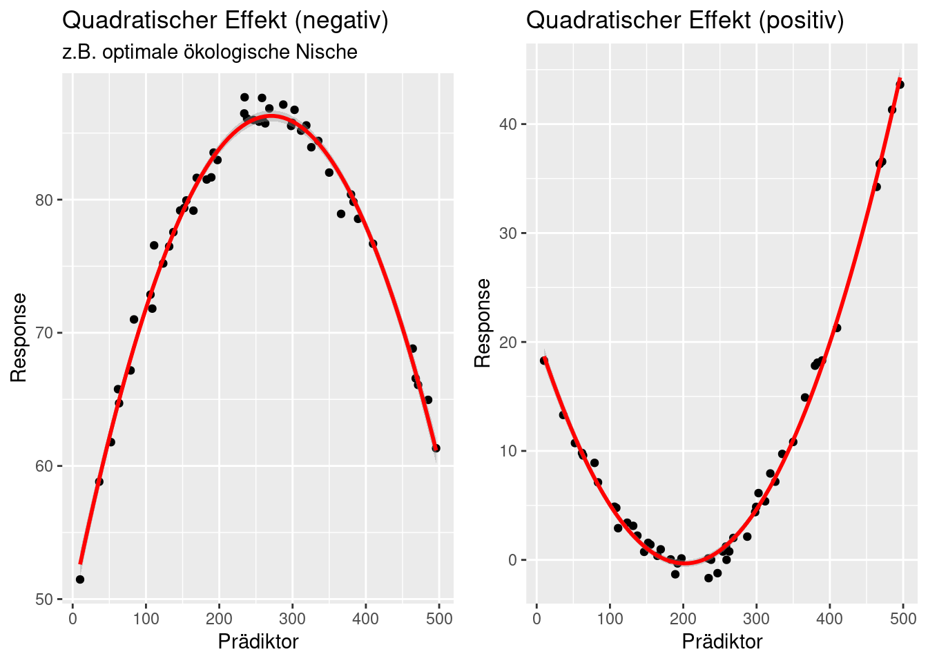
Figure 15.1: Quadratische Effekte.

Interaktionen beschreiben Situationen, bei denen der Effekt eines Prädiktors vom Wert eines anderen Prädiktors abhängt. Ein einfaches Beispiel ist Pflanzenwachstum. Pflanzen wachsen besser, wenn die Temperatur zunimmt ⁶⁰, Pflanzen wachsen auch besser, wenn mehr Wasser verfügbar ist⁶¹. Die Effekte sind jedoch nicht additiv. Wenn wir 30°C haben und kein Wasser ist der Effekt ein anderer als bei 30°C und ausreichend Wasser.

Während man bei rein additiven Haupteffekten den Zusammenhang zwischen 2 Prädiktoren und dem Response nur mit einer ebenen Fläche, die man im Raum rotiert darstellen kann, erlauben Interaktionen es, die Regressionsfläche zu verbiegen.

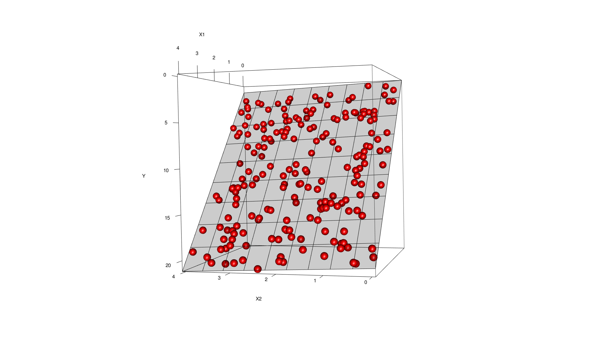
Regressiosnfläche für 2 Haupteffekte. Die Regressionsfläche ist eben, die Steigung kannn über die beiden Regressionskoeffizienten verändert werden..

Figure 15.2: Regressiosnfläche für 2 Haupteffekte. Die Regressionsfläche ist eben, die Steigung kannn über die beiden Regressionskoeffizienten verändert werden..

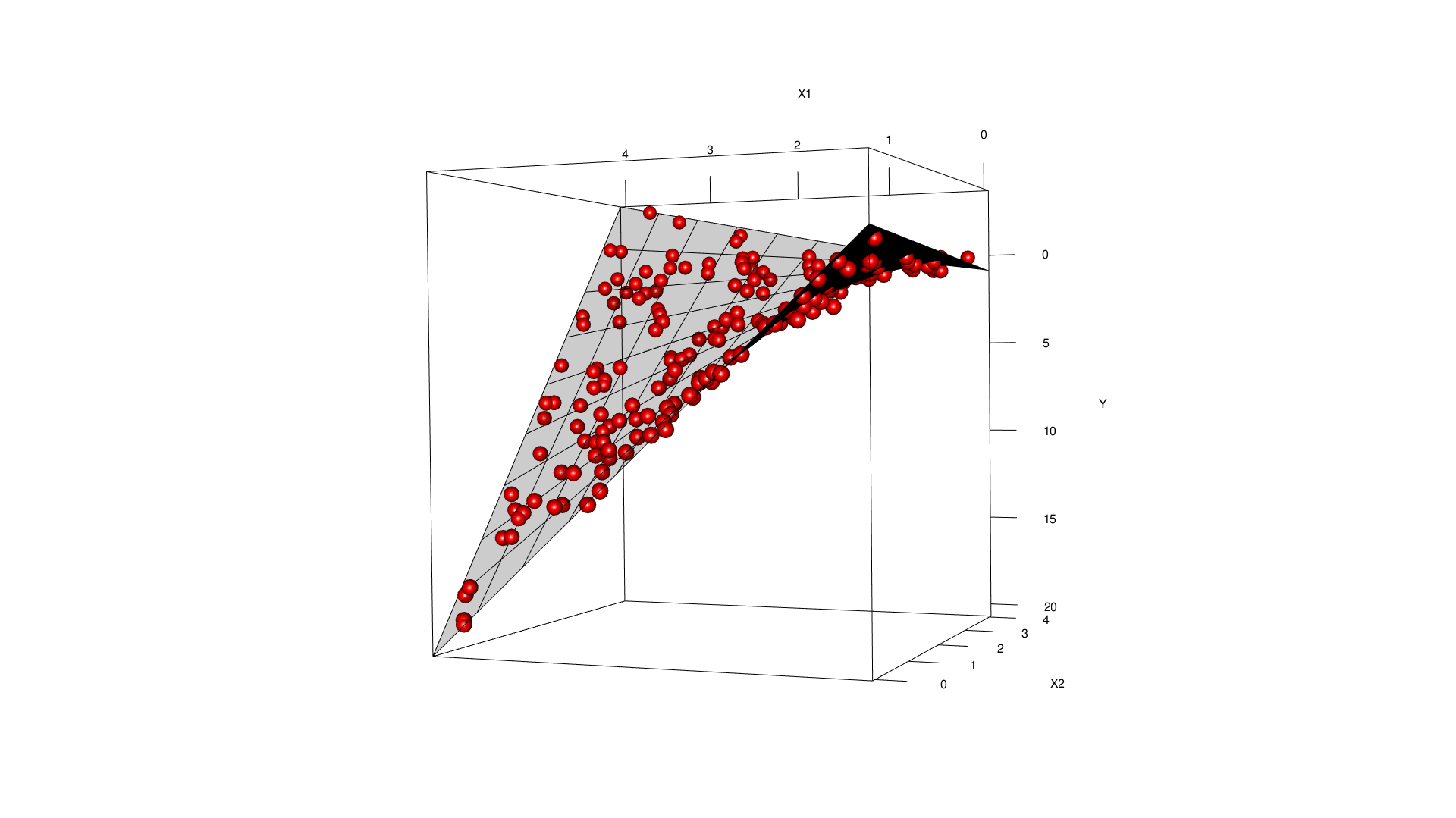
Figure 15.3: Interaktion zwischen den beiden Prädiktoren im Modell. Die Regressionsfläche ist gebogen.

15.2 Anwendungsbeispiel Temperaturdaten

Daten einlesen

temp <- read.table("data/temperatur.csv", header=TRUE)

15.2.1 Russland

Selektion von Stationen in Russland ohne NAs:

temp.ru <- subset(temp, CNTRY_NAME == "Russia")
temp.ru <- subset(temp.ru, ELEV > -20)
dim(temp.ru)

## [1] 50 36

Standardisieren von Länge und Breite:

temp.ru$LAT.cent <- temp.ru$LAT - mean(temp.ru$LAT)
temp.ru$LON.cent <- temp.ru$LON - mean(temp.ru$LON)

15.2.1.1 Polynomiale Effekt

Was ist mit quadratischen Effekten? Vielleicht wirken Längen- und Breitengrad ja auch quadratisch auf die Temperatur ein. Da der ^ Operator wir der + und der - und der * Operator überladen sind müssen wir den quadratischen Effekt entweder über I() oder über poly definieren. poly erzeugt dabei orthogonale Polygone, was i.d.R. von Vorteil ist.

Der Weg über I():

g <- lm(YEAR ~ ELEV+ I(ELEV^2) + LAT.cent + LON.cent, data=temp.ru)
summary(g)

## 
## Call:
## lm(formula = YEAR ~ ELEV + I(ELEV^2) + LAT.cent + LON.cent, data = temp.ru)
## 
## Residuals:
##      Min       1Q   Median       3Q      Max 
## -2.60096 -0.78573  0.06268  0.85677  2.36774 
## 
## Coefficients:
##               Estimate Std. Error t value Pr(>|t|)    
## (Intercept) -2.439e-01  3.184e-01  -0.766 0.447807    
## ELEV        -5.388e-03  1.387e-03  -3.884 0.000334 ***
## I(ELEV^2)    3.719e-07  7.858e-07   0.473 0.638318    
## LAT.cent    -7.845e-01  3.516e-02 -22.309  < 2e-16 ***
## LON.cent    -1.083e-01  1.154e-02  -9.384 3.66e-12 ***
## ---
## Signif. codes:  0 '***' 0.001 '**' 0.01 '*' 0.05 '.' 0.1 ' ' 1
## 
## Residual standard error: 1.252 on 45 degrees of freedom
## Multiple R-squared:  0.9337, Adjusted R-squared:  0.9278 
## F-statistic: 158.4 on 4 and 45 DF,  p-value: < 2.2e-16

Und nun über orthogonale Polynome mittels poly():

g.poly <- lm(YEAR ~ poly(ELEV,2) + LAT.cent + LON.cent, data=temp.ru)
summary(g.poly)

## 
## Call:
## lm(formula = YEAR ~ poly(ELEV, 2) + LAT.cent + LON.cent, data = temp.ru)
## 
## Residuals:
##      Min       1Q   Median       3Q      Max 
## -2.60096 -0.78573  0.06268  0.85677  2.36774 
## 
## Coefficients:
##                 Estimate Std. Error t value Pr(>|t|)    
## (Intercept)     -1.98438    0.17701 -11.211 1.29e-14 ***
## poly(ELEV, 2)1 -14.82349    1.52082  -9.747 1.15e-12 ***
## poly(ELEV, 2)2   0.65676    1.38774   0.473    0.638    
## LAT.cent        -0.78446    0.03516 -22.309  < 2e-16 ***
## LON.cent        -0.10827    0.01154  -9.384 3.66e-12 ***
## ---
## Signif. codes:  0 '***' 0.001 '**' 0.01 '*' 0.05 '.' 0.1 ' ' 1
## 
## Residual standard error: 1.252 on 45 degrees of freedom
## Multiple R-squared:  0.9337, Adjusted R-squared:  0.9278 
## F-statistic: 158.4 on 4 and 45 DF,  p-value: < 2.2e-16

Wie wir sehen, erhalten wir deutlich andere Koeffizientenschätzer bei den beiden Ansätzen.

Wir wollen hier zunächst einfach bei den nicht orthogonalen Polygonen bleiben. Um festzustellen, ob der quadratische Term das Modell signifikant verbessert verwenden wir die Hilfsfunktion drop1, der jeden möglichen Term entfernt und jeweils den AIC (oder den BIC, wenn k entsprechend gesetzt ist) berechnet.

drop1(g)

## Single term deletions
## 
## Model:
## YEAR ~ ELEV + I(ELEV^2) + LAT.cent + LON.cent
##           Df Sum of Sq    RSS     AIC
## <none>                  70.50  27.177
## ELEV       1     23.64  94.13  39.635
## I(ELEV^2)  1      0.35  70.85  25.425
## LAT.cent   1    779.67 850.17 149.671
## LON.cent   1    137.96 208.46  79.386

Wir sehen, dass der AIC um gut 2 Einheiten sinkt, wenn wir den quadratischen Term wieder entfernen. Ein deltaAIC von weniger als 2 (d.h. die Differenz zwischen 2 AIC Werten ist kleiner als 2) kann man als statistisch gleichwertige Modellgüten ansehen. Beide Modelle sind also in etwa gleich gut. Ich würde trotzdem das einfachere Modell bevorzugen.

Wichtig ist, das drop1 bei den quadratischen Effekten nicht automatisch das Marginalitätsprinzip respektiert. Wir müssen selbst dafür sorgen, dass es eingehalten wird, in dem wir keinen Haupteffekt aus dem Modell werfen, der in einem Term höherer Ordnung (oder einer Interaktion) enthalten ist.

Nun noch einaml mit dem BIC:

drop1(g, k = log(nrow(temp.ru)) )

## Single term deletions
## 
## Model:
## YEAR ~ ELEV + I(ELEV^2) + LAT.cent + LON.cent
##           Df Sum of Sq    RSS     AIC
## <none>                  70.50  36.737
## ELEV       1     23.64  94.13  47.283
## I(ELEV^2)  1      0.35  70.85  33.073
## LAT.cent   1    779.67 850.17 157.319
## LON.cent   1    137.96 208.46  87.034

Hier ist das Ergebnis eindeutig: der quadratische Term, trägt nicht signifikant zur Modellgüte bei.

Nun noch einmal für die orthogonalen Polygone - die Interpretation ist hier schwieriger, da die Gleichung nicht mehr einfach \(a + bx + cx^2\) ist, sondern zwei neue orthogonal zueinander stehende Variablen x’ und x’’ erzeugt werden. Dafür sind beide Koeffizienten nicht miteinander korreliert (orthogonal).

drop1(g.poly)

## Single term deletions
## 
## Model:
## YEAR ~ poly(ELEV, 2) + LAT.cent + LON.cent
##               Df Sum of Sq    RSS     AIC
## <none>                      70.50  27.177
## poly(ELEV, 2)  2    154.83 225.33  81.277
## LAT.cent       1    779.67 850.17 149.671
## LON.cent       1    137.96 208.46  79.386

Leider kann drop1 nur den ganzen rpoly(ELEV,2) Term auf einmal entfernen und nicht, wie gewünscht nur den Term 2. Ordnung. Deswegen müssen wir dies manuell machen.

g.poly2 <- update(g.poly, ~. -poly(ELEV,2) + poly(ELEV,1))
summary(g.poly2)

## 
## Call:
## lm(formula = YEAR ~ LAT.cent + LON.cent + poly(ELEV, 1), data = temp.ru)
## 
## Residuals:
##      Min       1Q   Median       3Q      Max 
## -2.46384 -0.76645  0.08496  0.77674  2.28727 
## 
## Coefficients:
##                Estimate Std. Error t value Pr(>|t|)    
## (Intercept)    -1.98438    0.17551 -11.306 7.11e-15 ***
## LAT.cent       -0.77774    0.03190 -24.378  < 2e-16 ***
## LON.cent       -0.10769    0.01138  -9.467 2.26e-12 ***
## poly(ELEV, 1) -14.64838    1.46263 -10.015 3.88e-13 ***
## ---
## Signif. codes:  0 '***' 0.001 '**' 0.01 '*' 0.05 '.' 0.1 ' ' 1
## 
## Residual standard error: 1.241 on 46 degrees of freedom
## Multiple R-squared:  0.9333, Adjusted R-squared:  0.929 
## F-statistic: 214.7 on 3 and 46 DF,  p-value: < 2.2e-16

Wenn wir das mit den Koeffizienten aus dem Modell mit den Haupteffekten ohne poly vergleichen, sehen wir, das der Koeffizient für ELEV unterschiedlich ist. Wie gesagt, es sind neue Hilfsvariablen. Beim Vorhersagen mit predict kommt trotzdem das gleich heraus. Einfacher ist es aber, in diesem Fall mit dem normalen Haupteffekt Modell g zu arbeiten.

AIC(g.poly)

## [1] 171.0707

AIC(g.poly2)

## [1] 169.319

15.2.1.2 Interaktionen

Nun wollen wir untersuchen, ob Interaktionen relevant sind. Der ^ Operator in einem formula-Objekt bewirkt, dass alle Interaktionen erster Ordnung zwischen den Prädiktoren in der Klammer berücksichtigt werden.

g <- lm(YEAR ~ (ELEV+  LAT.cent + LON.cent)^2, data=temp.ru)
summary(g)

## 
## Call:
## lm(formula = YEAR ~ (ELEV + LAT.cent + LON.cent)^2, data = temp.ru)
## 
## Residuals:
##     Min      1Q  Median      3Q     Max 
## -2.7112 -0.7016  0.1724  0.7027  2.3213 
## 
## Coefficients:
##                     Estimate Std. Error t value Pr(>|t|)    
## (Intercept)       -0.8374443  0.3924021  -2.134   0.0386 *  
## ELEV              -0.0005087  0.0021350  -0.238   0.8128    
## LAT.cent          -0.7603968  0.0326131 -23.316  < 2e-16 ***
## LON.cent          -0.0938562  0.0144875  -6.478 7.36e-08 ***
## ELEV:LAT.cent      0.0004796  0.0002566   1.869   0.0685 .  
## ELEV:LON.cent     -0.0002094  0.0001026  -2.041   0.0474 *  
## LAT.cent:LON.cent -0.0014476  0.0014300  -1.012   0.3171    
## ---
## Signif. codes:  0 '***' 0.001 '**' 0.01 '*' 0.05 '.' 0.1 ' ' 1
## 
## Residual standard error: 1.211 on 43 degrees of freedom
## Multiple R-squared:  0.9406, Adjusted R-squared:  0.9324 
## F-statistic: 113.6 on 6 and 43 DF,  p-value: < 2.2e-16

Wir sehen jede Menge nicht signifikanter Terme. Mittels drop1 ermitteln wir, welchen Term wir als erstes (niemals mehr als einen auf einmal entfernen, da sich alle Koeffizienten, Standardfehler und Signifikanzniveaus der anderen Terme dabei verändern) entfernen sollten.

drop1(g)

## Single term deletions
## 
## Model:
## YEAR ~ (ELEV + LAT.cent + LON.cent)^2
##                   Df Sum of Sq    RSS    AIC
## <none>                         63.076 25.616
## ELEV:LAT.cent      1    5.1234 68.199 27.521
## ELEV:LON.cent      1    6.1123 69.188 28.240
## LAT.cent:LON.cent  1    1.5032 64.579 24.794

Dies setzen wir am einfachsten mittels update um - der : Operator bezeichnet dabei die Interaktion zwischen den beiden beteiligten Haupteffekten:

g <- update(g, ~. -LAT.cent:LON.cent)
drop1(g)

## Single term deletions
## 
## Model:
## YEAR ~ ELEV + LAT.cent + LON.cent + ELEV:LAT.cent + ELEV:LON.cent
##               Df Sum of Sq    RSS    AIC
## <none>                     64.579 24.794
## ELEV:LAT.cent  1    3.6343 68.214 25.531
## ELEV:LON.cent  1    4.6515 69.231 26.271

Da der \(\delta\) AIC kleiner 2 ist würde ich weitere Terme entfernen:

g <- update(g, ~. -ELEV:LAT.cent)
drop1(g)

## Single term deletions
## 
## Model:
## YEAR ~ ELEV + LAT.cent + LON.cent + ELEV:LON.cent
##               Df Sum of Sq    RSS     AIC
## <none>                      68.21  25.531
## LAT.cent       1    824.86 893.07 152.132
## ELEV:LON.cent  1      2.63  70.85  25.425

g <- update(g, ~. -ELEV:LON.cent)
drop1(g)

## Single term deletions
## 
## Model:
## YEAR ~ ELEV + LAT.cent + LON.cent
##          Df Sum of Sq    RSS     AIC
## <none>                 70.85  25.425
## ELEV      1    154.48 225.33  81.277
## LAT.cent  1    915.28 986.13 155.088
## LON.cent  1    138.03 208.88  77.487

Hier sind wir am Ende angelangt.

Wir könnten den Ablauf auch über step durchführen, der drop1 und update automatisch aufruft.

g <- lm(YEAR ~ (ELEV+  LAT.cent + LON.cent)^2, data=temp.ru)
step(g)

## Start:  AIC=25.62
## YEAR ~ (ELEV + LAT.cent + LON.cent)^2
## 
##                     Df Sum of Sq    RSS    AIC
## - LAT.cent:LON.cent  1    1.5032 64.579 24.794
## <none>                           63.076 25.616
## - ELEV:LAT.cent      1    5.1234 68.199 27.521
## - ELEV:LON.cent      1    6.1123 69.188 28.240
## 
## Step:  AIC=24.79
## YEAR ~ ELEV + LAT.cent + LON.cent + ELEV:LAT.cent + ELEV:LON.cent
## 
##                 Df Sum of Sq    RSS    AIC
## <none>                       64.579 24.794
## - ELEV:LAT.cent  1    3.6343 68.214 25.531
## - ELEV:LON.cent  1    4.6515 69.231 26.271

## 
## Call:
## lm(formula = YEAR ~ ELEV + LAT.cent + LON.cent + ELEV:LAT.cent + 
##     ELEV:LON.cent, data = temp.ru)
## 
## Coefficients:
##   (Intercept)           ELEV       LAT.cent       LON.cent  ELEV:LAT.cent  
##    -0.5442916     -0.0019156     -0.7647990     -0.0916829      0.0003277  
## ELEV:LON.cent  
##    -0.0001658

Allerdings hört die Funktion hier zu früh auf, da das \(\delta\) AIC nicht beachtet wird.

15.2.2 Kanada

Durch seine geographische Lage (große Wasserkörper auf der westlichen und der östlichen Seite), könnte man für Kanada einen quadratischen Effekt hinsichtlich des Längengrades auf die Jahresmitteltemperatur vermuten, ggf. auch eine Interaktio.

Laden der Daten und fitten des Modells nur für die Haupteffekte

temp.ca <- temp %>% filter(CNTRY_NAME == "Canada")

g.ca <- lm(YEAR ~ ELEV+ LAT + LON, data = temp.ca)
summary(g.ca)

## 
## Call:
## lm(formula = YEAR ~ ELEV + LAT + LON, data = temp.ca)
## 
## Residuals:
##     Min      1Q  Median      3Q     Max 
## -3.9572 -1.1495 -0.1294  1.1152  4.3326 
## 
## Coefficients:
##               Estimate Std. Error t value Pr(>|t|)    
## (Intercept) 38.2020482  0.8110678  47.101  < 2e-16 ***
## ELEV        -0.0016589  0.0003874  -4.282 2.75e-05 ***
## LAT         -0.8760948  0.0161448 -54.265  < 2e-16 ***
## LON         -0.1007708  0.0057162 -17.629  < 2e-16 ***
## ---
## Signif. codes:  0 '***' 0.001 '**' 0.01 '*' 0.05 '.' 0.1 ' ' 1
## 
## Residual standard error: 1.636 on 224 degrees of freedom
## Multiple R-squared:  0.9311, Adjusted R-squared:  0.9301 
## F-statistic:  1009 on 3 and 224 DF,  p-value: < 2.2e-16

Test auf quadratischen Effekt

g.caPoly2 <- lm(YEAR ~ ELEV+ LAT + poly(LON,2), data = temp.ca)
summary(g.caPoly2)

## 
## Call:
## lm(formula = YEAR ~ ELEV + LAT + poly(LON, 2), data = temp.ca)
## 
## Residuals:
##     Min      1Q  Median      3Q     Max 
## -3.6671 -0.7819  0.0221  0.8009  4.2127 
## 
## Coefficients:
##                 Estimate Std. Error t value Pr(>|t|)    
## (Intercept)    4.822e+01  7.329e-01  65.794  < 2e-16 ***
## ELEV          -1.186e-03  3.172e-04  -3.739 0.000235 ***
## LAT           -8.862e-01  1.313e-02 -67.508  < 2e-16 ***
## poly(LON, 2)1 -3.429e+01  1.601e+00 -21.414  < 2e-16 ***
## poly(LON, 2)2  1.460e+01  1.347e+00  10.842  < 2e-16 ***
## ---
## Signif. codes:  0 '***' 0.001 '**' 0.01 '*' 0.05 '.' 0.1 ' ' 1
## 
## Residual standard error: 1.327 on 223 degrees of freedom
## Multiple R-squared:  0.9549, Adjusted R-squared:  0.9541 
## F-statistic:  1179 on 4 and 223 DF,  p-value: < 2.2e-16

Test auf Interaktion

g.caInt<- lm(YEAR ~ ELEV+ LAT *LON, data = temp.ca)
summary(g.caInt)

## 
## Call:
## lm(formula = YEAR ~ ELEV + LAT * LON, data = temp.ca)
## 
## Residuals:
##     Min      1Q  Median      3Q     Max 
## -3.9767 -1.0913  0.0173  1.0375  3.8072 
## 
## Coefficients:
##               Estimate Std. Error t value Pr(>|t|)    
## (Intercept) 26.7890324  3.5111135   7.630 6.77e-13 ***
## ELEV        -0.0019757  0.0003906  -5.058 8.86e-07 ***
## LAT         -0.6645984  0.0653200 -10.175  < 2e-16 ***
## LON         -0.2275634  0.0384071  -5.925 1.17e-08 ***
## LAT:LON      0.0023044  0.0006906   3.337 0.000993 ***
## ---
## Signif. codes:  0 '***' 0.001 '**' 0.01 '*' 0.05 '.' 0.1 ' ' 1
## 
## Residual standard error: 1.6 on 223 degrees of freedom
## Multiple R-squared:  0.9343, Adjusted R-squared:  0.9332 
## F-statistic: 793.4 on 4 and 223 DF,  p-value: < 2.2e-16

Test auf Interaktion mit quadratischem Effekt.

g.caIntPoly<- lm(YEAR ~ ELEV+ LAT * poly(LON,2), data = temp.ca)
summary(g.caIntPoly)

## 
## Call:
## lm(formula = YEAR ~ ELEV + LAT * poly(LON, 2), data = temp.ca)
## 
## Residuals:
##      Min       1Q   Median       3Q      Max 
## -2.67092 -0.60768  0.06757  0.67782  2.93637 
## 
## Coefficients:
##                     Estimate Std. Error t value Pr(>|t|)    
## (Intercept)        5.010e+01  6.043e-01  82.915  < 2e-16 ***
## ELEV              -1.635e-03  2.588e-04  -6.316 1.45e-09 ***
## LAT               -9.127e-01  1.067e-02 -85.582  < 2e-16 ***
## poly(LON, 2)1     -1.259e+02  9.437e+00 -13.342  < 2e-16 ***
## poly(LON, 2)2      5.534e+01  8.289e+00   6.676 1.96e-10 ***
## LAT:poly(LON, 2)1  1.635e+00  1.715e-01   9.533  < 2e-16 ***
## LAT:poly(LON, 2)2 -6.650e-01  1.501e-01  -4.430 1.48e-05 ***
## ---
## Signif. codes:  0 '***' 0.001 '**' 0.01 '*' 0.05 '.' 0.1 ' ' 1
## 
## Residual standard error: 1.053 on 221 degrees of freedom
## Multiple R-squared:  0.9718, Adjusted R-squared:  0.9711 
## F-statistic:  1271 on 6 and 221 DF,  p-value: < 2.2e-16

Vergleichen wir die Modelle einmal mittels AIC:

AIC(g.ca)

## [1] 877.5011

AIC(g.caPoly2)

## [1] 782.9726

AIC(g.caInt)

## [1] 868.3921

AIC(g.caIntPoly)

## [1] 679.3417

Das komplexe Modell wird favorisiert, da der AIC am kleinsten ist.

Um zu verstehen, wie die Zusammenhänge aussehen, müssen wir predict benutzen. Bereiten wir zunächst die Daten für die Vorhersage vor. expand.grid erstellt dabei alle möglichen Kombinationen der einzelnen Felder - wir wollen alles 3 Prädiktoren varieren. Allerdings verwenden wir für die Geländehöhe und den Längengrad nur 3 Werte, während wir für den Breitenkreis - der den stärksten Effekt hat - 100 Werte. Die Motivation liegt darin, wie wir die Zusammenhänge am Ende plotten wollen.

newdatCa <- expand.grid(ELEV = quantile(temp.ca$ELEV, 
                                        probs = c(.25, .5, .75)),
                        LAT = seq(min(temp.ca$LAT), 
                                  max(temp.ca$LAT), length.out = 100),
                        LON = quantile(temp.ca$LON, 
                                        probs = c(.25, .5, .75)))

Nun wenden wir predict an.

predMain <- predict(g.ca, newdata = newdatCa, interval = "confidenc") %>%
  as.data.frame()
predPoly2 <- predict(g.caPoly2, newdata = newdatCa, interval = "confidenc") %>%
  as.data.frame()
predInt <- predict(g.caInt, newdata = newdatCa, interval = "confidenc") %>%
  as.data.frame()
predIntPoly <- predict(g.caIntPoly, newdata = newdatCa, interval = "confidenc") %>%
  as.data.frame()

Die Vorhersage hängen wir für das Plotten an den data.frame mit den für die Vorhersage benutzten Werten für die Prädiktoren an.

newdatCa$predMain <- predMain$fit
newdatCa$predMain_lwr <- predMain$lwr
newdatCa$predMain_upr <- predMain$upr

newdatCa$predPoly <- predPoly2$fi
newdatCa$predPoly_lwr <- predPoly2$lwr
newdatCa$predPoly_upr <- predPoly2$upr

newdatCa$predInt <- predInt$fit
newdatCa$predInt_lwr <- predInt$lwr
newdatCa$predInt_upr <- predInt$upr

newdatCa$pred_quadIn <- predIntPoly$fit
newdatCa$pred_quadIn_lwr <- predIntPoly$lwr
newdatCa$pred_quadIn_upr <- predIntPoly$upr

Nun bringen wir den dat.frame vom weiten in ein langes Format für das Plotten mit ggplot2. Hierzu verwenden wir ein Pivotierungserkzeug, wie es aus der Einführung in die Geoinformatik bekannt sein dürfte.

prediction_long <- pivot_longer(newdatCa, cols = -(1:3))

idx_main <- grep(pattern = "Main", prediction_long$name)
idx_poly <- grep(pattern = "Poly", prediction_long$name)
idx_int <- grep(pattern = "Int", prediction_long$name)
idx_intpoly <- grep(pattern = "quadIn", prediction_long$name)

idx_lwr <- grep(pattern = "lwr", prediction_long$name)
idx_upr <- grep(pattern = "upr", prediction_long$name)

prediction_long$model <- "main"
prediction_long$model[idx_poly] <- "quadratic"
prediction_long$model[idx_int] <- "interaction"
prediction_long$model[idx_intpoly] <- "interaction quadratic"

prediction_long$type <- "fit"
prediction_long$type[idx_lwr] <- "lwr"
prediction_long$type[idx_upr] <- "upr"

Nun der eigentliche Plot

prediction_long%>% filter(type == "fit") %>%
ggplot( mapping = aes(
  x = LAT, y = value, lty = type, color = model)) +
  geom_line() +
  facet_wrap(~ LON + ELEV, labeller = label_both)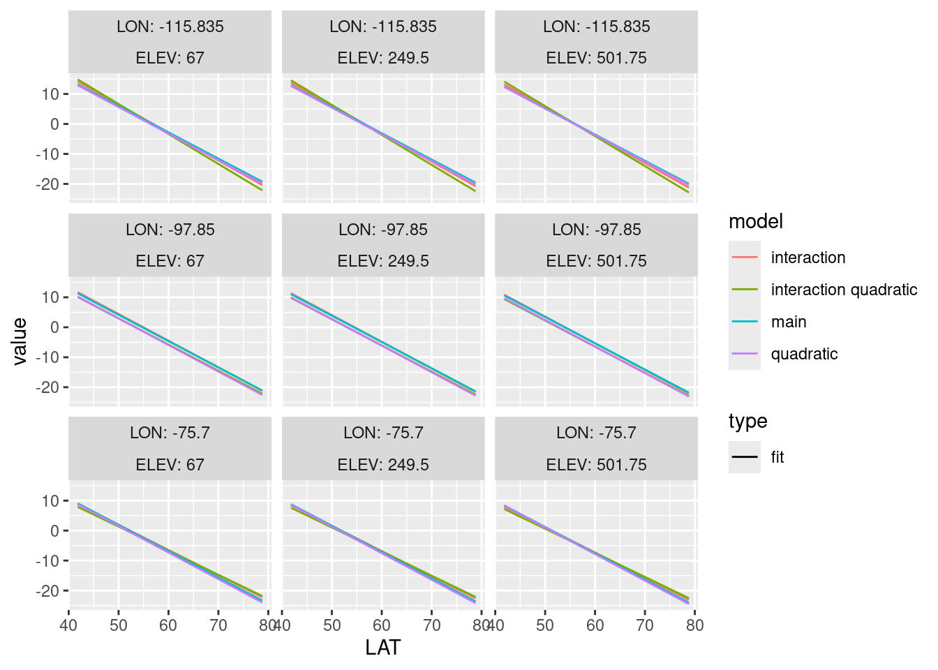

Wie wir sehen, haben wir nur sehr schwache nichtlineare Effekte im Modell. Signifikanz ist nicht das Gleiche wie Bedeutsamkeit.

15.2.3 All-subset Regression

Anstelle der stepwise regression wird oftmals die all-subset Regression empfohlen, die alle Kombinationen testet. Das Packet leaps übernimmt das für uns. Allerdings beachtet es dabei nicht das Prinzip der Marginalität und es kann nur für das lineare Modell eingesetzt werden.

Wir schauen uns dies einmal für die russischen Klimastationen an.

#####################################################
#### Using an all-subset-regression
#####################################################
require(leaps) # das Package muss vermutlich installiert werden

## Loading required package: leaps

subs <- regsubsets(YEAR ~ poly(ELEV,2) + poly(LAT.cent,2) + poly(LON.cent,2) , data=temp.ru, method="exhaustive", nbest=1)
(subs.s <- summary(subs))

## Subset selection object
## Call: regsubsets.formula(YEAR ~ poly(ELEV, 2) + poly(LAT.cent, 2) + 
##     poly(LON.cent, 2), data = temp.ru, method = "exhaustive", 
##     nbest = 1)
## 6 Variables  (and intercept)
##                    Forced in Forced out
## poly(ELEV, 2)1         FALSE      FALSE
## poly(ELEV, 2)2         FALSE      FALSE
## poly(LAT.cent, 2)1     FALSE      FALSE
## poly(LAT.cent, 2)2     FALSE      FALSE
## poly(LON.cent, 2)1     FALSE      FALSE
## poly(LON.cent, 2)2     FALSE      FALSE
## 1 subsets of each size up to 6
## Selection Algorithm: exhaustive
##          poly(ELEV, 2)1 poly(ELEV, 2)2 poly(LAT.cent, 2)1 poly(LAT.cent, 2)2
## 1  ( 1 ) " "            " "            "*"                " "               
## 2  ( 1 ) "*"            " "            "*"                " "               
## 3  ( 1 ) "*"            " "            "*"                " "               
## 4  ( 1 ) "*"            " "            "*"                "*"               
## 5  ( 1 ) "*"            " "            "*"                "*"               
## 6  ( 1 ) "*"            "*"            "*"                "*"               
##          poly(LON.cent, 2)1 poly(LON.cent, 2)2
## 1  ( 1 ) " "                " "               
## 2  ( 1 ) " "                " "               
## 3  ( 1 ) "*"                " "               
## 4  ( 1 ) "*"                " "               
## 5  ( 1 ) "*"                "*"               
## 6  ( 1 ) "*"                "*"

Im Plot sieht das viel übersichtlicher aus:

###################################################
### How does performance change with the number of parameters? 
###################################################
par(mfrow=c(2,2), mar=c(2.7,4.7,1,1), oma=c(2,0,0,0))
plot(1:6, subs.s$rsq, xlab="# Parameter", ylab=expression(R^2), pch=21, bg="blue", cex=1.5, type="b")
plot(1:6, subs.s$adjr2, xlab="# Parameter", ylab=expression(paste(sep="", R^2, ".adj")), pch=21, bg="blue", cex=1.5, type="b")
plot(1:6, subs.s$bic, xlab="# Parameter", ylab="BIC", pch=21, bg="blue", cex=1.5, type="b")
plot(1:6, subs.s$rss, xlab="# Parameter", ylab="RSS", pch=21, bg="blue", cex=1.5, type="b")
mtext(text = "# parameters", side = 1, line = 3, at = 0)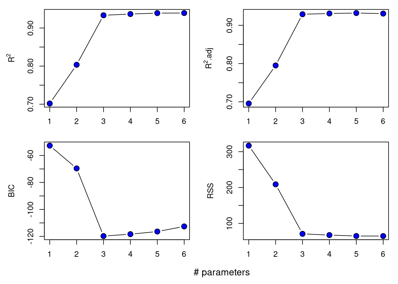

Das Modell mit 3 Parameter wird vom BIC favorisiert.

Nun wollen wir aber auch wissen, welche Variablen dabei im Modell sind:

###################################################
### which variables are in models with 1,2,3,... variables
### and how does the goodness-of-fit indicator react?
###################################################
par(mfrow=c(1,3), oma=c(3,0,0,0), mar=c(8.1, 1.1, .1,.1), cex.lab=1.4)
plot(subs)
plot(subs, scale="adjr2")
plot(subs, scale="r2")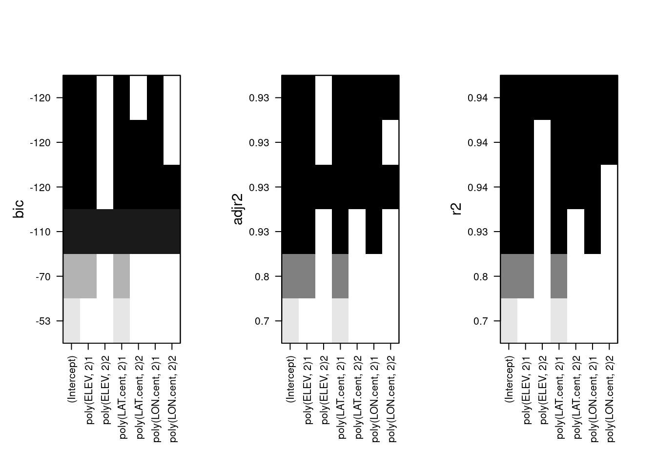

Wir können auch die Koeffizienten extrahieren - hier für die Modelle mit 1 bis 4 Parametern:

# coefficients for the best model for 4..8 predictors
coef(subs, 1:4)

## [[1]]
##        (Intercept) poly(LAT.cent, 2)1 
##          -1.984379         -27.311679 
## 
## [[2]]
##        (Intercept)     poly(ELEV, 2)1 poly(LAT.cent, 2)1 
##          -1.984379         -12.023801         -33.362243 
## 
## [[3]]
##        (Intercept)     poly(ELEV, 2)1 poly(LAT.cent, 2)1 poly(LON.cent, 2)1 
##          -1.984379         -14.648379         -43.173925         -14.672258 
## 
## [[4]]
##        (Intercept)     poly(ELEV, 2)1 poly(LAT.cent, 2)1 poly(LAT.cent, 2)2 
##          -1.984379         -14.532479         -42.087418          -2.348418 
## poly(LON.cent, 2)1 
##         -12.895568

Für das favorisierte 3 Parameter Modell sind wir also beim ursprünglichen Modell mit linearen Termen für Geländehöhe, Breitengrad und Längengrad.

Oder auch die Varianz-Covarianz-Matrix für die Regressionskoeffizienten ausgeben lassen - hier für das 1-Parameter Modell:

# variance-covariance matrix for the 1 parameter model
vcov(subs,1)

##                    (Intercept) poly(LAT.cent, 2)1
## (Intercept)          0.1320185           0.000000
## poly(LAT.cent, 2)1   0.0000000           6.600926

15.3 Anwendungsbeispiel CO2 Konzentrationen

Wir laden die athmosphärischen in situ Messungen der \(\textrm{CO}_2\) Konzentration am Standort Mauna Loa, Hawaii (Thoning, Crotwell, and Mund 2020), die bereits vorprozessiert und als Rdata Datei abgespeichert wurden ⁶². Der loadBefehl lädt die Rdata Datei und macht die gespeicherten (serialisierten) Objekte wieder verfügbar - hier den data.frame co2InSitu.

load("data/co2InSitu_MLO.Rdata")

Die Daten zeigen die bekannte Zunahme der athmosphärischen \(\textrm{CO}_2\) zusätzlich zu den - für diesen Breitengrad - typischen saisonalen Schankungen aufgrund der Vegetationsentwicklung auf.

ggplot(co2InSitu, mapping = aes(x=Date, y=value)) + geom_line() + 
  labs(title="C02 in situ Messungen", subtitle = "Mauna Loa, Hawaii, United States") + 
  xlab("") + ylab("CO2 [ppm]")

## Warning: Removed 501 rows containing missing values or values outside the scale range
## (`geom_line()`).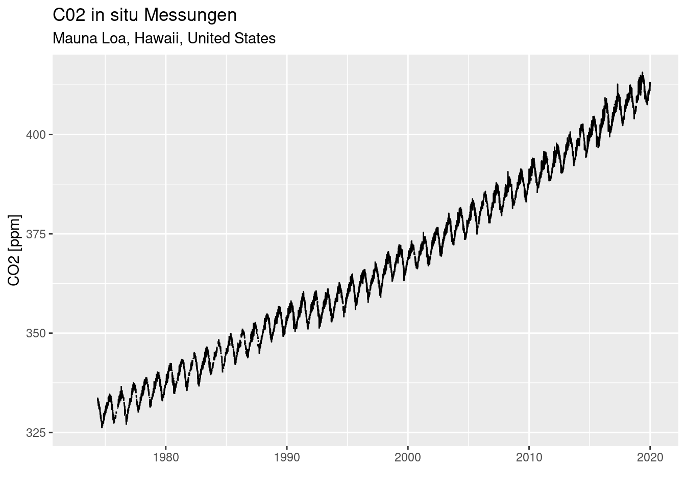

Wir können die Zunahme mit einem Polynom ersten oder zweiten Grades modellierten.

g1 <- lm(value ~ Date, data=co2InSitu)
g2 <- lm(value ~ poly(Date,2), data=co2InSitu)

Beide Modell unterscheiden sich nur unwesentlich hinsichtlich des adjustierten \(R^2\) Wertes. Sind sie trotzdem unterschiedlich hinsichtlich der Modelgüte?

summary(g1)

## 
## Call:
## lm(formula = value ~ Date, data = co2InSitu)
## 
## Residuals:
##     Min      1Q  Median      3Q     Max 
## -8.5595 -2.2804 -0.0345  2.1810 10.4171 
## 
## Coefficients:
##              Estimate Std. Error t value Pr(>|t|)    
## (Intercept) 3.182e+02  6.380e-02  4986.9   <2e-16 ***
## Date        5.631e-08  6.533e-11   861.8   <2e-16 ***
## ---
## Signif. codes:  0 '***' 0.001 '**' 0.01 '*' 0.05 '.' 0.1 ' ' 1
## 
## Residual standard error: 3.149 on 13944 degrees of freedom
##   (3220 observations deleted due to missingness)
## Multiple R-squared:  0.9816, Adjusted R-squared:  0.9816 
## F-statistic: 7.427e+05 on 1 and 13944 DF,  p-value: < 2.2e-16

summary(g2)

## 
## Call:
## lm(formula = value ~ poly(Date, 2), data = co2InSitu)
## 
## Residuals:
##    Min     1Q Median     3Q    Max 
## -6.580 -1.879  0.095  1.855  7.463 
## 
## Coefficients:
##                 Estimate Std. Error t value Pr(>|t|)    
## (Intercept)    3.655e+02  2.043e-02 17886.7   <2e-16 ***
## poly(Date, 2)1 3.108e+03  2.812e+00  1105.3   <2e-16 ***
## poly(Date, 2)2 2.863e+02  2.796e+00   102.4   <2e-16 ***
## ---
## Signif. codes:  0 '***' 0.001 '**' 0.01 '*' 0.05 '.' 0.1 ' ' 1
## 
## Residual standard error: 2.38 on 13943 degrees of freedom
##   (3220 observations deleted due to missingness)
## Multiple R-squared:  0.9895, Adjusted R-squared:  0.9895 
## F-statistic: 6.557e+05 on 2 and 13943 DF,  p-value: < 2.2e-16

Ein Modellvergleich mittels AIC zeigt klar, dass das Modell mit dem Polynom zweiten Grades den Verlauf deutlich besser beschreibt.

AIC(g1)

## [1] 71578.22

AIC(g2)

## [1] 63761.67

Ein likelihood-ratio-Test kommt zum gleichen klaren Ergebnis.

lmtest::lrtest(g1,g2)

## Likelihood ratio test
## 
## Model 1: value ~ Date
## Model 2: value ~ poly(Date, 2)
##   #Df LogLik Df  Chisq Pr(>Chisq)    
## 1   3 -35786                         
## 2   4 -31877  1 7818.6  < 2.2e-16 ***
## ---
## Signif. codes:  0 '***' 0.001 '**' 0.01 '*' 0.05 '.' 0.1 ' ' 1

Ein visueller Vergleich (Abbildung 15.4) zeigt ebenfalls, dass das Modell mit dem Polynom 2. Grades den Trend besser beschreibt als ein einfacher linearer Zusammenhang. Insbesondere trifft die Vorhersage die Werte zum Ende der Beobachtungsperiode besser als der einfache lineare Zusammenhang.

p1 <- ggplot(co2InSitu, mapping = aes(x=Date, y=value)) + geom_line() + 
  geom_smooth(method="lm", col="red") +
  labs(title="C02 in situ Messungen", subtitle = "Mauna Loa, Hawaii, United States - Poly1") + 
  xlab("") + ylab("CO2 [ppm]")

p2 <- ggplot(co2InSitu, mapping = aes(x=Date, y=value)) + geom_line() + 
  geom_smooth(method="lm", formula= y ~poly(x,2), col="red") +
  labs(title="C02 in situ Messungen", subtitle = "Mauna Loa, Hawaii, United States - Poly 2") + 
  xlab("") + ylab("CO2 [ppm]")

ggarrange(p1,p2)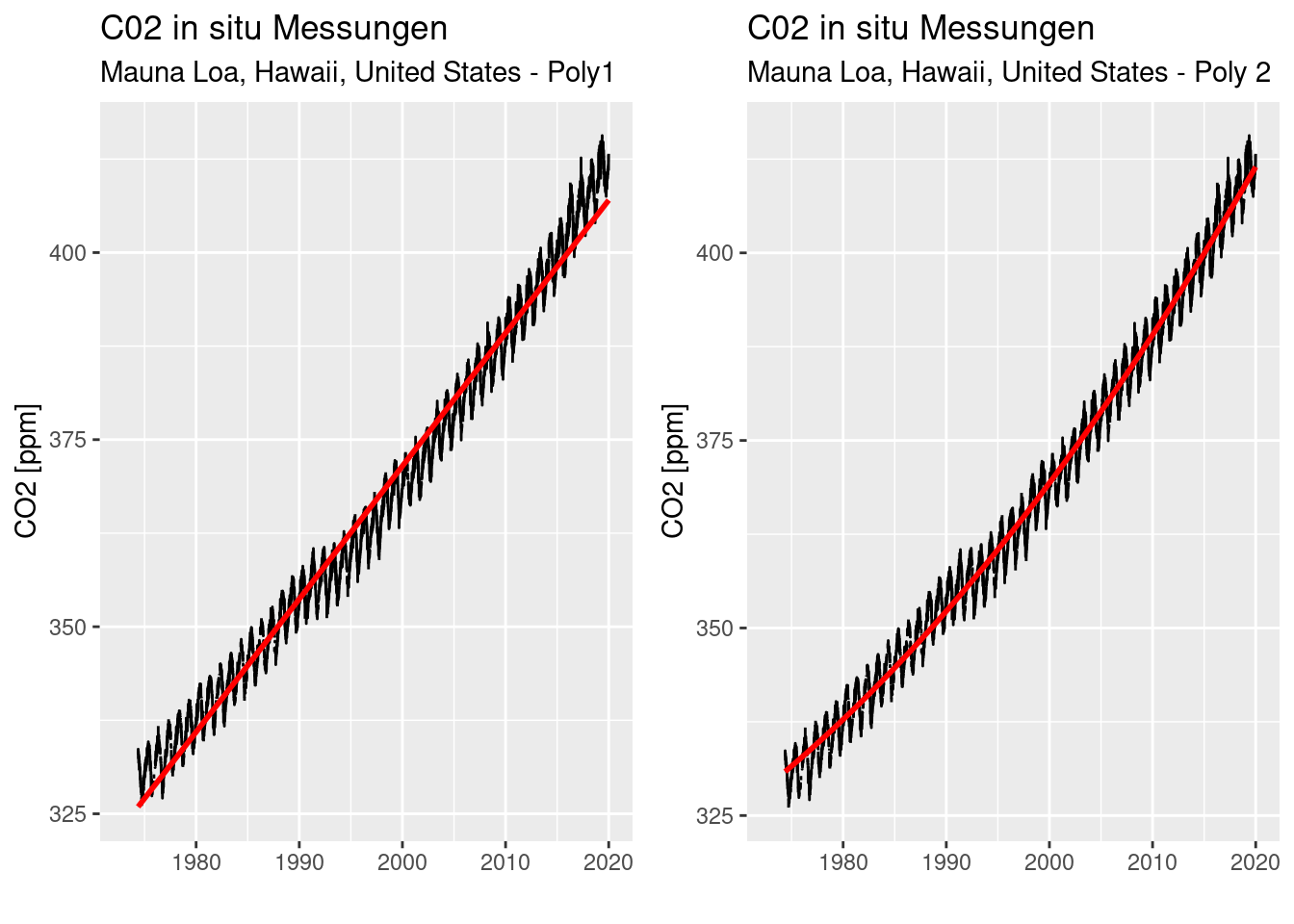

Vergleich eines inearen (links) und eines quadratischen (rechts) Vorhersagemodells für die athmosphärischen CO2 Konzentrationen am Standort Mauna Loa, Hawaii.

Figure 15.4: Vergleich eines inearen (links) und eines quadratischen (rechts) Vorhersagemodells für die athmosphärischen CO2 Konzentrationen am Standort Mauna Loa, Hawaii.

15.4 Anwendungsbeispiel Baumdichte und Klima

Bisher waren die Nichtlinearen Zusammenhänge eher nicht so überzeugend. Deswegen hier ein Beispiel, bei dem die Effekte bedeutsam sind.

Interaktionen und polynome Terme testen wir anhand eines Datensatzes von Anadón, Sala, and Maestre (2014). Der Datensatz enthält Informationen zur Baumdichte in Lateinamerika sowie klimatische Prädiktoren.

dat <- read.table("data/10Mpoints_database_Anadonetal2014JECOL.txt", header=TRUE)

summary(dat)

##        X                 Y                BIO1             BIO12       
##  Min.   :-176.55   Min.   :-55.141   Min.   :-273.24   Min.   :   0.0  
##  1st Qu.:-108.89   1st Qu.: -4.733   1st Qu.: -44.00   1st Qu.: 309.3  
##  Median : -85.09   Median : 41.384   Median :  70.90   Median : 611.4  
##  Mean   : -89.17   Mean   : 29.502   Mean   :  71.95   Mean   : 876.5  
##  3rd Qu.: -66.85   3rd Qu.: 59.887   3rd Qu.: 209.00   3rd Qu.:1225.6  
##  Max.   : -34.98   Max.   : 83.013   Max.   : 288.00   Max.   :9431.2  
##       PET              MOD44B           GLC        
##  Min.   :  49.96   Min.   : 0.00   Min.   : 1.000  
##  1st Qu.: 477.40   1st Qu.: 0.00   1st Qu.: 4.000  
##  Median : 982.40   Median : 3.58   Median :12.000  
##  Mean   :1002.31   Mean   :17.81   Mean   : 9.639  
##  3rd Qu.:1578.20   3rd Qu.:27.86   3rd Qu.:14.000  
##  Max.   :2078.52   Max.   :84.05   Max.   :22.000

Die Daten liegen in einem regelmäßigen Raster vor. Folgende Attributwerte sind für uns im weiteren relevant.

MOD44B enthält den aus MODIS Fernerkundungsdaten abgeleiteten Flächendeckungsgrad von Bäumen (Tree cover [%*100]) je Rasterzelle.
BIO1 - enthält die mittlere Jahrestemperatur der Zelle (Annual Mean Temperature)
BIO12 - enthält die Jahressumme der Niederschläge in der Zelle (Annual Precipitation)
GLC - sind Landnutzungsdaten aufgrund der Global land cover Datensatzes.

Wir wollen uns hier mit dem Zusammenhang zwischen Baumbedeckungsgrad und Klimavariablen in allen Zellen beschäftigen, die zu LN-Klasse 2 (GLC == 2: Tree cover, broadleaved,deciduous, closed, Closed cover > 40%) gehören.

Die Selektion führe ich mittels des subset durch.

dat.glc2 <- subset(dat, GLC ==2)

Bevor wir uns an die Analyse machen, teilen wir die Daten in einen Trainings- und einen Validierungsdatensatz auf. Damit können wir eine bessere Vorhersage hinsichtlich des Vorhersagefehlers auf unbekannten Daten erhalten (Generalisierungsfehler).

Damit wir immer dieselben Aufteilung verwenden setze ich den Zufallszahlengenerator auf einen fixen Wert

set.seed(42)
n <- nrow(dat.glc2)
idx_test <- sample(x = 1:n, size = 0.2*n, replace = FALSE)

dat.glc2_test <- dat.glc2[idx_test,]
dat.glc2_train <- dat.glc2[-idx_test,]

dim(dat.glc2_test)

## [1] 108   7

dim(dat.glc2_train)

## [1] 432   7

15.4.1 Explorative Analyse

source("functions/pairsPannelFunctions.r")

pairs(dat.glc2_train[, c("MOD44B", "BIO1", "BIO12")], lower.panel = panel.smooth, diag.panel = panel.hist, upper.panel = panel.cor, labels = c("Baumbedeckung", "Temperatur", "Niederschlag"), las=1)

15.4.2 Haupteffekte

g.main <- lm(MOD44B ~ BIO1 + BIO12 , data=dat.glc2_train)
summary(g.main)

## 
## Call:
## lm(formula = MOD44B ~ BIO1 + BIO12, data = dat.glc2_train)
## 
## Residuals:
##     Min      1Q  Median      3Q     Max 
## -47.946  -9.491   1.474  11.593  44.659 
## 
## Coefficients:
##              Estimate Std. Error t value Pr(>|t|)    
## (Intercept) 31.161520   2.463819  12.648   <2e-16 ***
## BIO1        -0.114719   0.009870 -11.622   <2e-16 ***
## BIO12        0.020586   0.002109   9.763   <2e-16 ***
## ---
## Signif. codes:  0 '***' 0.001 '**' 0.01 '*' 0.05 '.' 0.1 ' ' 1
## 
## Residual standard error: 16.55 on 429 degrees of freedom
## Multiple R-squared:  0.3034, Adjusted R-squared:  0.3002 
## F-statistic: 93.43 on 2 and 429 DF,  p-value: < 2.2e-16

Wir sehen, dass der Baumbedeckungsgrad mit zunehmender Temperatur abnimmt und mit zunehmendem Niederschlag zunimmt.

Plotten wir das in der üblichen Form.

Zunächst erstelle ich insgesamt sechs data.frames in dem ich jeweils Temperatur oder Niederschlag festhalte und den anderen Wert auf einem konstanten Wert halte.

summary(dat.glc2_train$BIO12)

##    Min. 1st Qu.  Median    Mean 3rd Qu.    Max. 
##   167.3   820.5  1058.6  1061.7  1241.3  3000.1

summary(dat.glc2_train$BIO1)

##    Min. 1st Qu.  Median    Mean 3rd Qu.    Max. 
##   -49.0    63.7   129.8   139.5   220.2   274.9

newD.prcp <- data.frame(BIO1 = mean(dat.glc2_train$BIO1), BIO12 = seq(min(dat.glc2_train$BIO12), max(dat.glc2_train$BIO12), length.out=100))
newD.prcp.t60 <- data.frame(BIO1 = 60, BIO12 = seq(min(dat.glc2_train$BIO12), max(dat.glc2_train$BIO12), length.out=100))
newD.prcp.t250 <- data.frame(BIO1 = 250, BIO12 = seq(min(dat.glc2_train$BIO12), max(dat.glc2_train$BIO12), length.out=100))

newD.temp <- data.frame(BIO12 = mean(dat.glc2_train$BIO12), BIO1 = seq(min(dat.glc2_train$BIO1), max(dat.glc2_train$BIO1), length.out=100))
newD.temp.p600 <- data.frame(BIO12 = 600, BIO1 = seq(min(dat.glc2_train$BIO1), max(dat.glc2_train$BIO1), length.out=100))
newD.temp.p1400 <- data.frame(BIO12 = 1400, BIO1 = seq(min(dat.glc2_train$BIO1), max(dat.glc2_train$BIO1), length.out=100))

Dann die Vorhersage für die sechs data.frames.

pred.prcp.main <- as.data.frame(predict(g.main, newdata = newD.prcp, interval="confidence"))
pred.prcp.t60.main <- as.data.frame(predict(g.main, newdata = newD.prcp.t60, interval="confidence"))
pred.prcp.t250.main <- as.data.frame(predict(g.main, newdata = newD.prcp.t250, interval="confidence"))

pred.temp.main <- as.data.frame(predict(g.main, newdata = newD.temp, interval="confidence"))
pred.temp.p600.main <- as.data.frame(predict(g.main, newdata = newD.temp.p600, interval="confidence"))
pred.temp.p1400.main <- as.data.frame(predict(g.main, newdata = newD.temp.p1400, interval="confidence"))

Dann plotte ich die jeweils die drei Regressionslinien für konstanten Niederschlag.

plot(MOD44B ~ BIO1, data=dat.glc2_train, las=1, pch=16, col=rgb(0,0,1,.25), xlab="Jahresmitteltemperatur [°C/10]", ylab="Baumbedeckungsgrad [%]", xlim=c(-52, 400), main="Haupteffekte", cex=.1+ sqrt( BIO12)/20)
lines(pred.temp.main$fit ~ newD.temp$BIO1, col="red", lwd=2)
lines(pred.temp.main$upr ~ newD.temp$BIO1, col="red", lty=2, lwd=2)
lines(pred.temp.main$lwr ~ newD.temp$BIO1, col="red", lty=2, lwd=2)

lines(pred.temp.p600.main$fit ~ newD.temp$BIO1, col="orange", lwd=2)
lines(pred.temp.p600.main$upr ~ newD.temp$BIO1, col="orange", lty=2, lwd=2)
lines(pred.temp.p600.main$lwr ~ newD.temp$BIO1, col="orange", lty=2, lwd=2)

lines(pred.temp.p1400.main$fit ~ newD.temp$BIO1, col="firebrick4", lwd=2)
lines(pred.temp.p1400.main$upr ~ newD.temp$BIO1, col="firebrick4", lty=2, lwd=2)
lines(pred.temp.p1400.main$lwr ~ newD.temp$BIO1, col="firebrick4", lty=2, lwd=2)

legend(x="right", legend=c("600", "1057.1", "1400"), title = "Jahresniederschlag", col=c("orange", "red", "firebrick4"), lwd=2, bty='n')

prcpVals <- c(600, 1000, 1400)
legend(x=320, y=28, legend=paste(prcpVals, "mm"), pt.cex=.1+ sqrt(prcpVals)/20, pch=16, col="blue", bty='n')

Und nun halten wir die Temperatur konstant und variieren den Niederschlag für den Plot.

plot(MOD44B ~ BIO12, data=dat.glc2_train, las=1, pch=16, col=rgb(0,0,1,.25), xlab="Jahresniederschlag [mm]", ylab="Baumbedeckungsgrad [%]", xlim=c(0, 4000), main="Haupteffekte", cex=.1+ sqrt(52+BIO1)/10)
lines(pred.prcp.main$fit ~ newD.prcp$BIO12, col="red", lwd=2)
lines(pred.prcp.main$upr ~ newD.prcp$BIO12, col="red", lty=2, lwd=2)
lines(pred.prcp.main$lwr ~ newD.prcp$BIO12, col="red", lty=2, lwd=2)

lines(pred.prcp.t60.main$fit ~ newD.prcp$BIO12, col="orange", lwd=2)
lines(pred.prcp.t60.main$upr ~ newD.prcp$BIO12, col="orange", lty=2, lwd=2)
lines(pred.prcp.t60.main$lwr ~ newD.prcp$BIO12, col="orange", lty=2, lwd=2)

lines(pred.prcp.t250.main$fit ~ newD.prcp$BIO12, col="firebrick4", lwd=2)
lines(pred.prcp.t250.main$upr ~ newD.prcp$BIO12, col="firebrick4", lty=2, lwd=2)
lines(pred.prcp.t250.main$lwr ~ newD.prcp$BIO12, col="firebrick4", lty=2, lwd=2)

legend(x=3200, y=60, legend=c("6", "14", "25"), title = "Jahresmittel-\ntemperatur [°C]", col=c("orange", "red", "firebrick4"), lwd=2, bty='n')
tempVals <- seq(-5, 30, by=10)
legend(x=3400, y=30, legend=paste(tempVals, "°C"), pt.cex=.1+ sqrt(52+tempVals*10)/10, pch=16, col="blue", bty='n')

15.4.3 Interaktionen

Gibt es Wechselwirkungen zwischen Temperatur und Niederschlag?

g.int <- lm(MOD44B ~ BIO1 * BIO12, data=dat.glc2_train)
summary(g.int)

## 
## Call:
## lm(formula = MOD44B ~ BIO1 * BIO12, data = dat.glc2_train)
## 
## Residuals:
##     Min      1Q  Median      3Q     Max 
## -68.367  -9.909  -0.632   9.905  43.315 
## 
## Coefficients:
##               Estimate Std. Error t value Pr(>|t|)    
## (Intercept) -9.620e+00  4.321e+00  -2.226   0.0265 *  
## BIO1         1.033e-01  2.178e-02   4.745 2.84e-06 ***
## BIO12        6.337e-02  4.336e-03  14.615  < 2e-16 ***
## BIO1:BIO12  -2.250e-04  2.058e-05 -10.932  < 2e-16 ***
## ---
## Signif. codes:  0 '***' 0.001 '**' 0.01 '*' 0.05 '.' 0.1 ' ' 1
## 
## Residual standard error: 14.65 on 428 degrees of freedom
## Multiple R-squared:  0.4555, Adjusted R-squared:  0.4516 
## F-statistic: 119.3 on 3 and 428 DF,  p-value: < 2.2e-16

Ja. Temperatur hat einen positiven Effekt auf Baumbedeckungsgrad, ebenso Niederschlag. Mit zunehmender Temperatur wird allerdings der Effekt von Niederschlag negativ (und umgekehrt).

Um das Modellverhalten besser verstehen zu können verwenden wir wieder predict und plotten dann wieder das Modellverhalten.

pred.prcp.int <- as.data.frame(predict(g.int, newdata = newD.prcp, interval="confidence"))
pred.prcp.t60.int <- as.data.frame(predict(g.int, newdata = newD.prcp.t60, interval="confidence"))
pred.prcp.t250.int <- as.data.frame(predict(g.int, newdata = newD.prcp.t250, interval="confidence"))

pred.temp.int <- as.data.frame(predict(g.int, newdata = newD.temp, interval="confidence"))
pred.temp.p600.int <- as.data.frame(predict(g.int, newdata = newD.temp.p600, interval="confidence"))
pred.temp.p1400.int <- as.data.frame(predict(g.int, newdata = newD.temp.p1400, interval="confidence"))

plot(MOD44B ~ BIO1, data=dat.glc2_train, las=1, pch=16, col=rgb(0,0,1,.25), xlab="Jahresmitteltemperatur [°C/10]", ylab="Baumbedeckungsgrad [%]", xlim=c(-52, 400), main="Interaktionen", cex=.1+ sqrt( BIO12)/20)
lines(pred.temp.int$fit ~ newD.temp$BIO1, col="red", lwd=2)
lines(pred.temp.int$upr ~ newD.temp$BIO1, col="red", lty=2, lwd=2)
lines(pred.temp.int$lwr ~ newD.temp$BIO1, col="red", lty=2, lwd=2)

lines(pred.temp.p600.int$fit ~ newD.temp$BIO1, col="orange", lwd=2)
lines(pred.temp.p600.int$upr ~ newD.temp$BIO1, col="orange", lty=2, lwd=2)
lines(pred.temp.p600.int$lwr ~ newD.temp$BIO1, col="orange", lty=2, lwd=2)

lines(pred.temp.p1400.int$fit ~ newD.temp$BIO1, col="firebrick4", lwd=2)
lines(pred.temp.p1400.int$upr ~ newD.temp$BIO1, col="firebrick4", lty=2, lwd=2)
lines(pred.temp.p1400.int$lwr ~ newD.temp$BIO1, col="firebrick4", lty=2, lwd=2)

legend(x="right", legend=c("600", "1057.1", "1400"), title = "Jahresniederschlag", col=c("orange", "red", "firebrick4"), lwd=2, bty='n')
legend(x=320, y=28, legend=paste(prcpVals, "mm"), pt.cex=.1+ sqrt(prcpVals)/20, pch=16, col="blue", bty='n')

Wie wir sehen verändert sich nicht nur der offset, sondern auch die Steigung der Regressionslinie für Baumbedeckung gegen Temperatur mit dem Jahresniederschlag. Höhere Jahresniederschläge haben einen positiven Effekt auf den Baumbedeckungsgrad, allerdings sinkt der Bedeckungsgrad zugleich stärker bei zunehmender Temperatur.

plot(MOD44B ~ BIO12, data=dat.glc2_train, las=1, pch=16, col=rgb(0,0,1,.25), xlab="Jahresniederschlag [mm]", ylab="Baumbedeckungsgrad [%]", xlim=c(0, 4000), main="Interaktion", cex=.1+ sqrt(52+BIO1)/10)
lines(pred.prcp.int$fit ~ newD.prcp$BIO12, col="red", lwd=2)
lines(pred.prcp.int$upr ~ newD.prcp$BIO12, col="red", lty=2, lwd=2)
lines(pred.prcp.int$lwr ~ newD.prcp$BIO12, col="red", lty=2, lwd=2)

lines(pred.prcp.t60.int$fit ~ newD.prcp$BIO12, col="orange", lwd=2)
lines(pred.prcp.t60.int$upr ~ newD.prcp$BIO12, col="orange", lty=2, lwd=2)
lines(pred.prcp.t60.int$lwr ~ newD.prcp$BIO12, col="orange", lty=2, lwd=2)

lines(pred.prcp.t250.int$fit ~ newD.prcp$BIO12, col="firebrick4", lwd=2)
lines(pred.prcp.t250.int$upr ~ newD.prcp$BIO12, col="firebrick4", lty=2, lwd=2)
lines(pred.prcp.t250.int$lwr ~ newD.prcp$BIO12, col="firebrick4", lty=2, lwd=2)

legend(x="right", legend=c("6", "14", "25"), title = "Jahresmittel-\ntemperatur [°C]", col=c("orange", "red", "firebrick4"), lwd=2, bty='n')
tempVals <- seq(-5, 30, by=10)
legend(x=3400, y=30, legend=paste(tempVals, "°C"), pt.cex=.1+ sqrt(52+tempVals*10)/10, pch=16, col="blue", bty='n')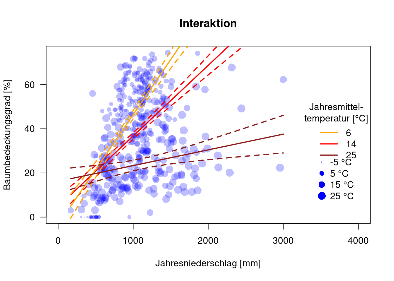

15.4.4 Polynomiale Terme

Polynomiale Terme erzeugen wir mittels poly. Der Parameter gibt an, welchen Grades das Polynom sein soll. Wenn wir von einer optimalen Klimanische ausgehen, wären quadratische Terme sinnvoll.

g.poly <- lm(MOD44B ~ poly(BIO1,2) + poly(BIO12,2), data=dat.glc2_train)
summary(g.poly)

## 
## Call:
## lm(formula = MOD44B ~ poly(BIO1, 2) + poly(BIO12, 2), data = dat.glc2_train)
## 
## Residuals:
##     Min      1Q  Median      3Q     Max 
## -44.216 -10.083   0.272  10.699  42.868 
## 
## Coefficients:
##                 Estimate Std. Error t value Pr(>|t|)    
## (Intercept)       37.014      0.735  50.361  < 2e-16 ***
## poly(BIO1, 2)1  -180.976     15.999 -11.312  < 2e-16 ***
## poly(BIO1, 2)2   -79.535     16.666  -4.772 2.50e-06 ***
## poly(BIO12, 2)1  154.043     15.822   9.736  < 2e-16 ***
## poly(BIO12, 2)2  -82.730     16.834  -4.915 1.27e-06 ***
## ---
## Signif. codes:  0 '***' 0.001 '**' 0.01 '*' 0.05 '.' 0.1 ' ' 1
## 
## Residual standard error: 15.28 on 427 degrees of freedom
## Multiple R-squared:  0.4094, Adjusted R-squared:  0.4038 
## F-statistic: 73.99 on 4 and 427 DF,  p-value: < 2.2e-16

Alle Terme sind signifikant.

Vorhersage mit den bereits vordefinierten data frames.

pred.prcp.poly <- as.data.frame(predict(g.poly, newdata = newD.prcp, interval="confidence"))
pred.prcp.t60.poly <- as.data.frame(predict(g.poly, newdata = newD.prcp.t60, interval="confidence"))
pred.prcp.t250.poly <- as.data.frame(predict(g.poly, newdata = newD.prcp.t250, interval="confidence"))

pred.temp.poly <- as.data.frame(predict(g.poly, newdata = newD.temp, interval="confidence"))
pred.temp.p600.poly <- as.data.frame(predict(g.poly, newdata = newD.temp.p600, interval="confidence"))
pred.temp.p1400.poly <- as.data.frame(predict(g.poly, newdata = newD.temp.p1400, interval="confidence"))

Plotten der Zusammenhänge

plot(MOD44B ~ BIO1, data=dat.glc2_train, las=1, pch=16, col=rgb(0,0,1,.25), xlab="Jahresmitteltemperatur [°C/10]", ylab="Baumbedeckungsgrad [%]", xlim=c(-52, 400), main="Polynome 2. Grades", cex=.1+ sqrt( BIO12)/20)
lines(pred.temp.poly$fit ~ newD.temp$BIO1, col="red", lwd=2)
lines(pred.temp.poly$upr ~ newD.temp$BIO1, col="red", lty=2, lwd=2)
lines(pred.temp.poly$lwr ~ newD.temp$BIO1, col="red", lty=2, lwd=2)

lines(pred.temp.p600.poly$fit ~ newD.temp$BIO1, col="orange", lwd=2)
lines(pred.temp.p600.poly$upr ~ newD.temp$BIO1, col="orange", lty=2, lwd=2)
lines(pred.temp.p600.poly$lwr ~ newD.temp$BIO1, col="orange", lty=2, lwd=2)

lines(pred.temp.p1400.poly$fit ~ newD.temp$BIO1, col="firebrick4", lwd=2)
lines(pred.temp.p1400.poly$upr ~ newD.temp$BIO1, col="firebrick4", lty=2, lwd=2)
lines(pred.temp.p1400.poly$lwr ~ newD.temp$BIO1, col="firebrick4", lty=2, lwd=2)

legend(x="right", legend=c("600", "1057.1", "1400"), title = "Jahresniederschlag", col=c("orange", "red", "firebrick4"), lwd=2, bty='n')
legend(x=320, y=28, legend=paste(prcpVals, "mm"), pt.cex=.1+ sqrt(prcpVals)/20, pch=16, col="blue", bty='n')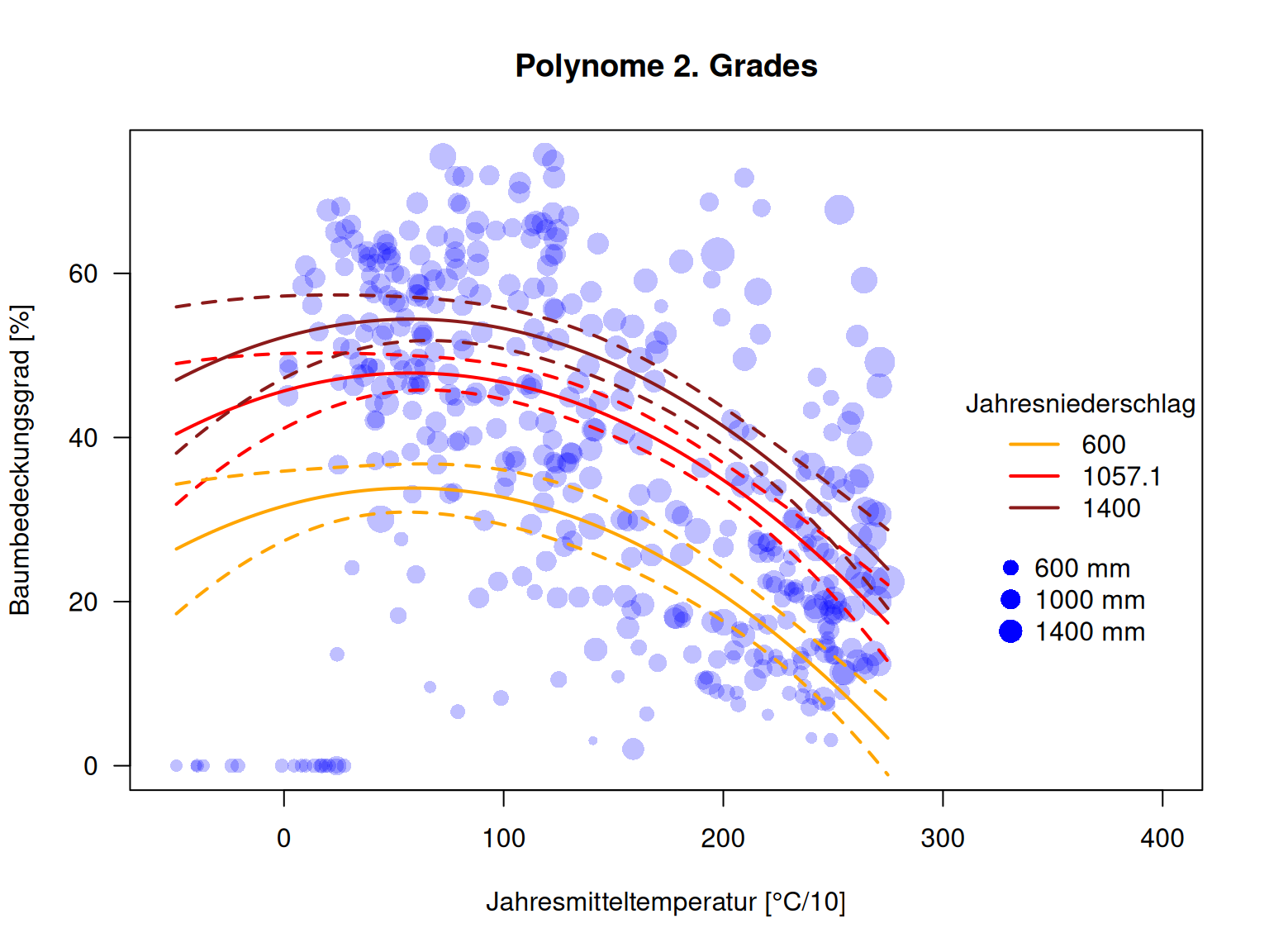

plot(MOD44B ~ BIO12, data=dat.glc2_train, las=1, pch=16, col=rgb(0,0,1,.25), xlab="Jahresniederschlag [mm]", ylab="Baumbedeckungsgrad [%]", xlim=c(0, 4000), main="Polynome 2. Grades", cex=.1+ sqrt(52+BIO1)/10)
lines(pred.prcp.poly$fit ~ newD.prcp$BIO12, col="red", lwd=2)
lines(pred.prcp.poly$upr ~ newD.prcp$BIO12, col="red", lty=2, lwd=2)
lines(pred.prcp.poly$lwr ~ newD.prcp$BIO12, col="red", lty=2, lwd=2)

lines(pred.prcp.t60.poly$fit ~ newD.prcp$BIO12, col="orange", lwd=2)
lines(pred.prcp.t60.poly$upr ~ newD.prcp$BIO12, col="orange", lty=2, lwd=2)
lines(pred.prcp.t60.poly$lwr ~ newD.prcp$BIO12, col="orange", lty=2, lwd=2)

lines(pred.prcp.t250.poly$fit ~ newD.prcp$BIO12, col="firebrick4", lwd=2)
lines(pred.prcp.t250.poly$upr ~ newD.prcp$BIO12, col="firebrick4", lty=2, lwd=2)
lines(pred.prcp.t250.poly$lwr ~ newD.prcp$BIO12, col="firebrick4", lty=2, lwd=2)

legend(x="right", legend=c("6", "14", "25"), title = "Jahresmittel-\ntemperatur [°C]", col=c("orange", "red", "firebrick4"), lwd=2, bty='n')
tempVals <- seq(-5, 30, by=10)
legend(x=3400, y=30, legend=paste(tempVals, "°C"), pt.cex=.1+ sqrt(52+tempVals*10)/10, pch=16, col="blue", bty='n')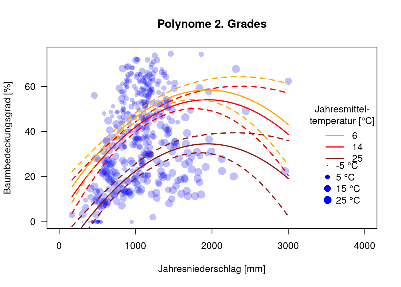

Wir sehen, dass bei hohen Niederschlagsmengen die Unsicherheit aufgrund der geringen Datendichte sehr hoch ist.

15.4.5 Polynomiale Terme und Interaktionen

g.int.poly <- lm(MOD44B ~ poly(BIO1,2) * poly(BIO12,2), data=dat.glc2_train)
summary(g.int.poly)

## 
## Call:
## lm(formula = MOD44B ~ poly(BIO1, 2) * poly(BIO12, 2), data = dat.glc2_train)
## 
## Residuals:
##     Min      1Q  Median      3Q     Max 
## -55.199  -9.403  -0.710   8.980  43.793 
## 
## Coefficients:
##                                 Estimate Std. Error t value Pr(>|t|)    
## (Intercept)                      36.1750     0.7982  45.320  < 2e-16 ***
## poly(BIO1, 2)1                 -193.4915    17.7601 -10.895  < 2e-16 ***
## poly(BIO1, 2)2                  -12.5650    17.0523  -0.737  0.46162    
## poly(BIO12, 2)1                 109.0577    24.2838   4.491 9.16e-06 ***
## poly(BIO12, 2)2                -174.4439    25.9143  -6.732 5.48e-11 ***
## poly(BIO1, 2)1:poly(BIO12, 2)1   12.1722   545.4537   0.022  0.98221    
## poly(BIO1, 2)2:poly(BIO12, 2)1 -891.6913   391.6951  -2.276  0.02332 *  
## poly(BIO1, 2)1:poly(BIO12, 2)2 3698.6353   544.0595   6.798 3.62e-11 ***
## poly(BIO1, 2)2:poly(BIO12, 2)2 -955.8178   275.6678  -3.467  0.00058 ***
## ---
## Signif. codes:  0 '***' 0.001 '**' 0.01 '*' 0.05 '.' 0.1 ' ' 1
## 
## Residual standard error: 13.58 on 423 degrees of freedom
## Multiple R-squared:  0.5374, Adjusted R-squared:  0.5287 
## F-statistic: 61.43 on 8 and 423 DF,  p-value: < 2.2e-16

drop1(g.int.poly, k=log(nrow(dat.glc2_train)))

## Single term deletions
## 
## Model:
## MOD44B ~ poly(BIO1, 2) * poly(BIO12, 2)
##                              Df Sum of Sq   RSS    AIC
## <none>                                    78037 2299.5
## poly(BIO1, 2):poly(BIO12, 2)  4     21606 99643 2380.8

Der BIC empfiehlt, die Interaktion im Modell zu lassen.

Vorhersage

pred.prcp.int.poly <- as.data.frame(predict(g.int.poly, newdata = newD.prcp, interval="confidence"))
pred.prcp.t60.int.poly <- as.data.frame(predict(g.int.poly, newdata = newD.prcp.t60, interval="confidence"))
pred.prcp.t250.int.poly <- as.data.frame(predict(g.int.poly, newdata = newD.prcp.t250, interval="confidence"))

pred.temp.int.poly <- as.data.frame(predict(g.int.poly, newdata = newD.temp, interval="confidence"))
pred.temp.p600.int.poly <- as.data.frame(predict(g.int.poly, newdata = newD.temp.p600, interval="confidence"))
pred.temp.p1400.int.poly <- as.data.frame(predict(g.int.poly, newdata = newD.temp.p1400, interval="confidence"))

Plotten der Zusammenhänge

plot(MOD44B ~ BIO1, data=dat.glc2_train, las=1, pch=16, col=rgb(0,0,1,.25), xlab="Jahresmitteltemperatur [°C/10]", ylab="Baumbedeckungsgrad [%]", xlim=c(-52, 400), main="Interaktion und Polynome 2. Grades", cex=.1+ sqrt( BIO12)/20)
lines(pred.temp.int.poly$fit ~ newD.temp$BIO1, col="red", lwd=2)
lines(pred.temp.int.poly$upr ~ newD.temp$BIO1, col="red", lty=2, lwd=2)
lines(pred.temp.int.poly$lwr ~ newD.temp$BIO1, col="red", lty=2, lwd=2)

lines(pred.temp.p600.int.poly$fit ~ newD.temp$BIO1, col="orange", lwd=2)
lines(pred.temp.p600.int.poly$upr ~ newD.temp$BIO1, col="orange", lty=2, lwd=2)
lines(pred.temp.p600.int.poly$lwr ~ newD.temp$BIO1, col="orange", lty=2, lwd=2)

lines(pred.temp.p1400.int.poly$fit ~ newD.temp$BIO1, col="firebrick4", lwd=2)
lines(pred.temp.p1400.int.poly$upr ~ newD.temp$BIO1, col="firebrick4", lty=2, lwd=2)
lines(pred.temp.p1400.int.poly$lwr ~ newD.temp$BIO1, col="firebrick4", lty=2, lwd=2)

legend(x="right", legend=c("600", "1057.1", "1400"), title = "Jahresniederschlag", col=c("orange", "red", "firebrick4"), lwd=2, bty='n')
legend(x=320, y=28, legend=paste(prcpVals, "mm"), pt.cex=.1+ sqrt(prcpVals)/20, pch=16, col="blue", bty='n')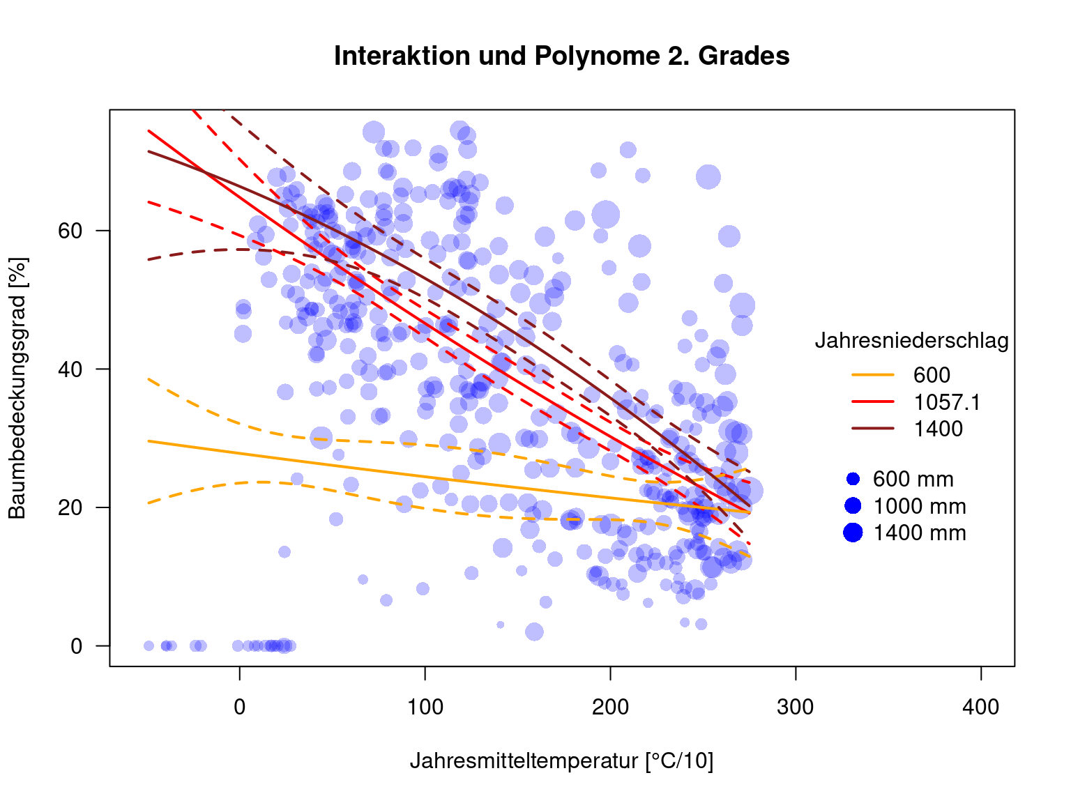

plot(MOD44B ~ BIO12, data=dat.glc2_train, las=1, pch=16, col=rgb(0,0,1,.25), xlab="Jahresniederschlag [mm]", ylab="Baumbedeckungsgrad [%]", xlim=c(0, 4000), main="Interaktion und Polynome 2. Grades", cex=.1+ sqrt(52+BIO1)/10)
lines(pred.prcp.int.poly$fit ~ newD.prcp$BIO12, col="red", lwd=2)
lines(pred.prcp.int.poly$upr ~ newD.prcp$BIO12, col="red", lty=2, lwd=2)
lines(pred.prcp.int.poly$lwr ~ newD.prcp$BIO12, col="red", lty=2, lwd=2)

lines(pred.prcp.t60.int.poly$fit ~ newD.prcp$BIO12, col="orange", lwd=2)
lines(pred.prcp.t60.int.poly$upr ~ newD.prcp$BIO12, col="orange", lty=2, lwd=2)
lines(pred.prcp.t60.int.poly$lwr ~ newD.prcp$BIO12, col="orange", lty=2, lwd=2)

lines(pred.prcp.t250.int.poly$fit ~ newD.prcp$BIO12, col="firebrick4", lwd=2)
lines(pred.prcp.t250.int.poly$upr ~ newD.prcp$BIO12, col="firebrick4", lty=2, lwd=2)
lines(pred.prcp.t250.int.poly$lwr ~ newD.prcp$BIO12, col="firebrick4", lty=2, lwd=2)

legend(x="right", legend=c("6", "14", "25"), title = "Jahresmittel-\ntemperatur [°C]", col=c("orange", "red", "firebrick4"), lwd=2, bty='n')
tempVals <- seq(-5, 30, by=10)
legend(x=3400, y=30, legend=paste(tempVals, "°C"), pt.cex=.1+ sqrt(52+tempVals*10)/10, pch=16, col="blue", bty='n')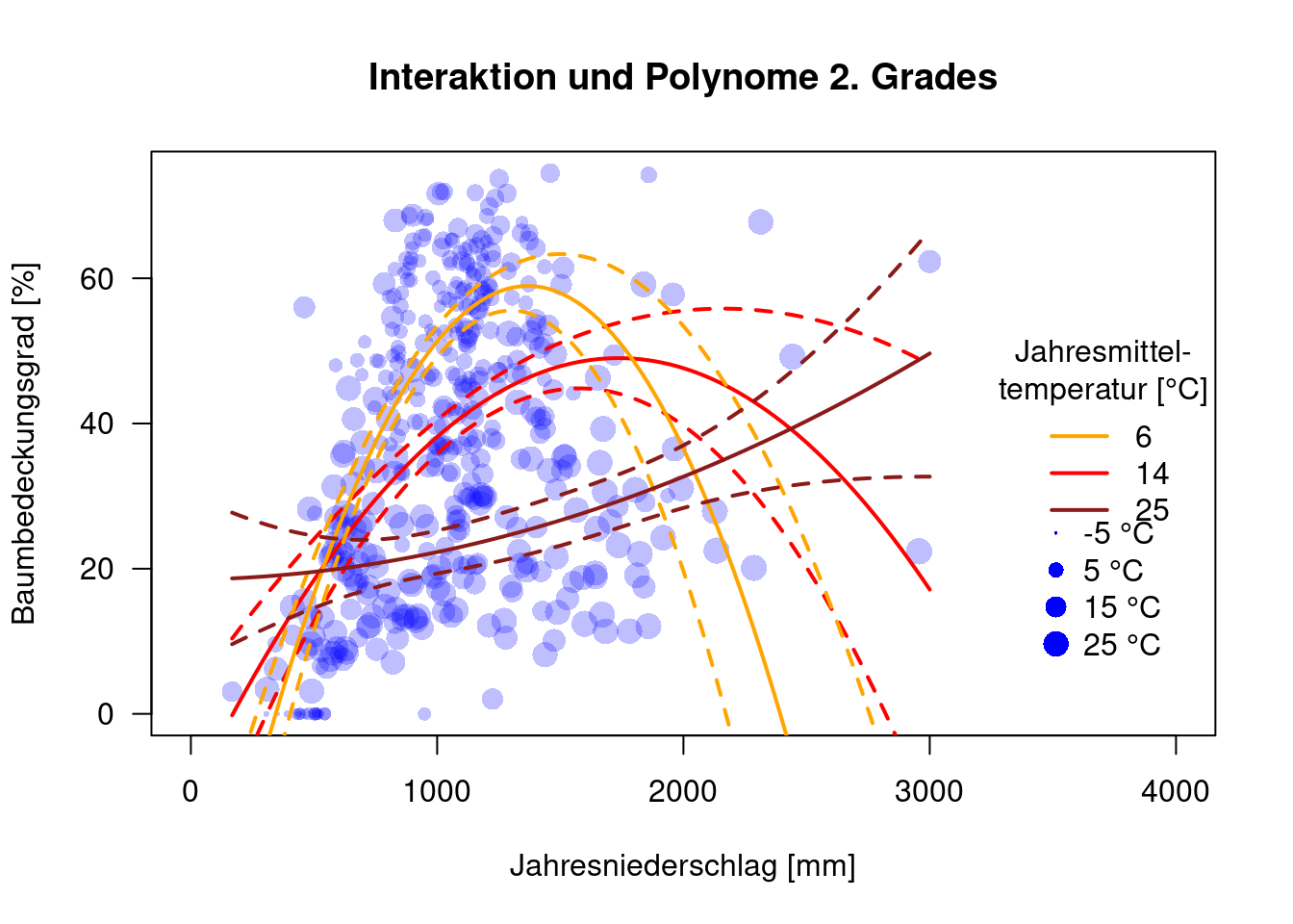

Für hohe Jahresniederschläge haben wir etwas wenig Daten, so dass mir die Kurvenverläufe für hohe Temperaturen nicht gut gefallen.

15.4.6 Polynomiale Terme und Interaktionen

g.int.polyPrc <- lm(MOD44B ~ BIO1 * poly(BIO12,2), data=dat.glc2_train)
summary(g.int.polyPrc)

## 
## Call:
## lm(formula = MOD44B ~ BIO1 * poly(BIO12, 2), data = dat.glc2_train)
## 
## Residuals:
##     Min      1Q  Median      3Q     Max 
## -52.978  -9.451  -1.155   9.330  43.319 
## 
## Coefficients:
##                        Estimate Std. Error t value Pr(>|t|)    
## (Intercept)           5.396e+01  1.500e+00  35.982  < 2e-16 ***
## BIO1                 -1.236e-01  8.866e-03 -13.946  < 2e-16 ***
## poly(BIO12, 2)1       2.485e+02  4.794e+01   5.183 3.38e-07 ***
## poly(BIO12, 2)2      -3.586e+02  4.614e+01  -7.770 5.91e-14 ***
## BIO1:poly(BIO12, 2)1 -7.593e-01  2.139e-01  -3.549 0.000429 ***
## BIO1:poly(BIO12, 2)2  1.505e+00  2.043e-01   7.368 9.08e-13 ***
## ---
## Signif. codes:  0 '***' 0.001 '**' 0.01 '*' 0.05 '.' 0.1 ' ' 1
## 
## Residual standard error: 13.74 on 426 degrees of freedom
## Multiple R-squared:  0.5231, Adjusted R-squared:  0.5175 
## F-statistic: 93.47 on 5 and 426 DF,  p-value: < 2.2e-16

drop1(g.int.polyPrc, k=log(nrow(dat.glc2_train)))

## Single term deletions
## 
## Model:
## MOD44B ~ BIO1 * poly(BIO12, 2)
##                     Df Sum of Sq    RSS    AIC
## <none>                            80448 2294.4
## BIO1:poly(BIO12, 2)  2     24510 104958 2397.2

Der BIC empfiehlt, die Interaktion im Modell zu lassen.

Vorhersage

pred.prcp.int.poly.prc <- as.data.frame(predict(g.int.polyPrc, newdata = newD.prcp, interval="confidence"))
pred.prcp.t60.int.poly.prc <- as.data.frame(predict(g.int.polyPrc, newdata = newD.prcp.t60, interval="confidence"))
pred.prcp.t250.int.poly.prc <- as.data.frame(predict(g.int.polyPrc, newdata = newD.prcp.t250, interval="confidence"))

pred.temp.int.poly.prc <- as.data.frame(predict(g.int.polyPrc, newdata = newD.temp, interval="confidence"))
pred.temp.p600.int.poly.prc <- as.data.frame(predict(g.int.polyPrc, newdata = newD.temp.p600, interval="confidence"))
pred.temp.p1400.int.poly.prc <- as.data.frame(predict(g.int.polyPrc, newdata = newD.temp.p1400, interval="confidence"))

Plotten der Zusammenhänge

plot(MOD44B ~ BIO1, data=dat.glc2_train, las=1, pch=16, col=rgb(0,0,1,.25), xlab="Jahresmitteltemperatur [°C/10]", ylab="Baumbedeckungsgrad [%]", xlim=c(-52, 400), main="Interaktion und Polynome 2. Grades", cex=.1+ sqrt( BIO12)/20)
lines(pred.temp.int.poly.prc$fit ~ newD.temp$BIO1, col="red", lwd=2)
lines(pred.temp.int.poly.prc$upr ~ newD.temp$BIO1, col="red", lty=2, lwd=2)
lines(pred.temp.int.poly.prc$lwr ~ newD.temp$BIO1, col="red", lty=2, lwd=2)

lines(pred.temp.p600.int.poly.prc$fit ~ newD.temp$BIO1, col="orange", lwd=2)
lines(pred.temp.p600.int.poly.prc$upr ~ newD.temp$BIO1, col="orange", lty=2, lwd=2)
lines(pred.temp.p600.int.poly.prc$lwr ~ newD.temp$BIO1, col="orange", lty=2, lwd=2)

lines(pred.temp.p1400.int.poly.prc$fit ~ newD.temp$BIO1, col="firebrick4", lwd=2)
lines(pred.temp.p1400.int.poly.prc$upr ~ newD.temp$BIO1, col="firebrick4", lty=2, lwd=2)
lines(pred.temp.p1400.int.poly.prc$lwr ~ newD.temp$BIO1, col="firebrick4", lty=2, lwd=2)

legend(x="right", legend=c("600", "1057.1", "1400"), title = "Jahresniederschlag", col=c("orange", "red", "firebrick4"), lwd=2, bty='n')
legend(x=320, y=28, legend=paste(prcpVals, "mm"), pt.cex=.1+ sqrt(prcpVals)/20, pch=16, col="blue", bty='n')

plot(MOD44B ~ BIO12, data=dat.glc2_train, las=1, pch=16, col=rgb(0,0,1,.25), xlab="Jahresniederschlag [mm]", ylab="Baumbedeckungsgrad [%]", xlim=c(0, 4000), main="Interaktion und Polynome 2. Grades", cex=.1+ sqrt(52+BIO1)/10)
lines(pred.prcp.int.poly.prc$fit ~ newD.prcp$BIO12, col="red", lwd=2)
lines(pred.prcp.int.poly.prc$upr ~ newD.prcp$BIO12, col="red", lty=2, lwd=2)
lines(pred.prcp.int.poly.prc$lwr ~ newD.prcp$BIO12, col="red", lty=2, lwd=2)

lines(pred.prcp.t60.int.poly.prc$fit ~ newD.prcp$BIO12, col="orange", lwd=2)
lines(pred.prcp.t60.int.poly.prc$upr ~ newD.prcp$BIO12, col="orange", lty=2, lwd=2)
lines(pred.prcp.t60.int.poly.prc$lwr ~ newD.prcp$BIO12, col="orange", lty=2, lwd=2)

lines(pred.prcp.t250.int.poly.prc$fit ~ newD.prcp$BIO12, col="firebrick4", lwd=2)
lines(pred.prcp.t250.int.poly.prc$upr ~ newD.prcp$BIO12, col="firebrick4", lty=2, lwd=2)
lines(pred.prcp.t250.int.poly.prc$lwr ~ newD.prcp$BIO12, col="firebrick4", lty=2, lwd=2)

legend(x="right", legend=c("6", "14", "25"), title = "Jahresmittel-\ntemperatur [°C]", col=c("orange", "red", "firebrick4"), lwd=2, bty='n')
tempVals <- seq(-5, 30, by=10)
legend(x=3400, y=28, legend=paste(tempVals, "°C"), pt.cex=.1+ sqrt(52+tempVals*10)/10, pch=16, col="blue", bty='n')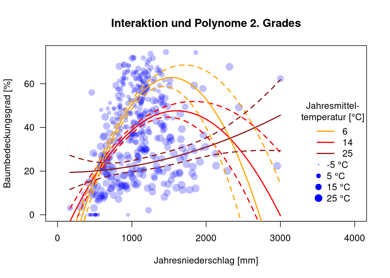

Mann könnte auch überlegen, die Interaktion nur zwischen den beiden Haupteffekten zuzulassen.

15.4.7 Generalisierungsfehler

Nun wollen wir aufgrundlage des Testdatensatzes den Generalisierungsfehler betrachten und schauen, ob die Modelle auch mit unbekannten Daten klarkommt. In einer realen Anwendung müsste man sich zudem um die räunmliche Autokorrelation kümmern, was die Signifikanzniveaus aber auch den Generalisierungs negativ verändern dürfte.

test.main <- predict(g.main, newdata = dat.glc2_test)
test.poly <- predict(g.poly, newdata = dat.glc2_test)
test.int <- predict(g.int, newdata = dat.glc2_test)
test.int.poly <- predict(g.int.poly, newdata = dat.glc2_test)
test.int.polyPrc <- predict(g.int.polyPrc, newdata = dat.glc2_test)


train.main <- predict(g.main, newdata = dat.glc2_train)
train.poly <- predict(g.poly, newdata = dat.glc2_train)
train.int <- predict(g.int, newdata = dat.glc2_train)
train.int.poly <- predict(g.int.poly, newdata = dat.glc2_train)
train.int.polyPrc <- predict(g.int.polyPrc, newdata = dat.glc2_train)

Funktion zum Berechnen des root mean square errors (der Quadratwurzel des mittleren quadrierten Fehlers):

rsme <- function(obs, pred)
{
  mse <- mean((obs-pred)^2)
  return(sqrt(mse))
}

res <- data.frame(model=c("Haupteffekte", "Interaktion", "Polynom 2. Grades", "Quadratisch &\nInteraktion", "Niederschlag quadartisch,\n Temperatur und Interaktion"), rsmeTrain = NA, rsmeTest=NA)

res$rsmeTest[1] <- rsme(dat.glc2_test$MOD44B, test.main)
res$rsmeTest[2] <- rsme(dat.glc2_test$MOD44B, test.int)
res$rsmeTest[3] <- rsme(dat.glc2_test$MOD44B, test.poly)
res$rsmeTest[4] <- rsme(dat.glc2_test$MOD44B, test.int.poly)
res$rsmeTest[5] <- rsme(dat.glc2_test$MOD44B, test.int.polyPrc)

res$rsmeTrain[1] <- rsme(dat.glc2_train$MOD44B, train.main)
res$rsmeTrain[2] <- rsme(dat.glc2_train$MOD44B, train.int)
res$rsmeTrain[3] <- rsme(dat.glc2_train$MOD44B, train.poly)
res$rsmeTrain[4] <- rsme(dat.glc2_train$MOD44B, train.int.poly)
res$rsmeTrain[5] <- rsme(dat.glc2_train$MOD44B, train.int.polyPrc)

Je kleiner der RSME, desto besser.

ggplot(data= res, mapping = aes(x= model, y= rsmeTest)) +
  geom_point() +
  coord_flip() + ylab("RSME") + xlab("") +
  labs(title = "Validierungsdatensatz")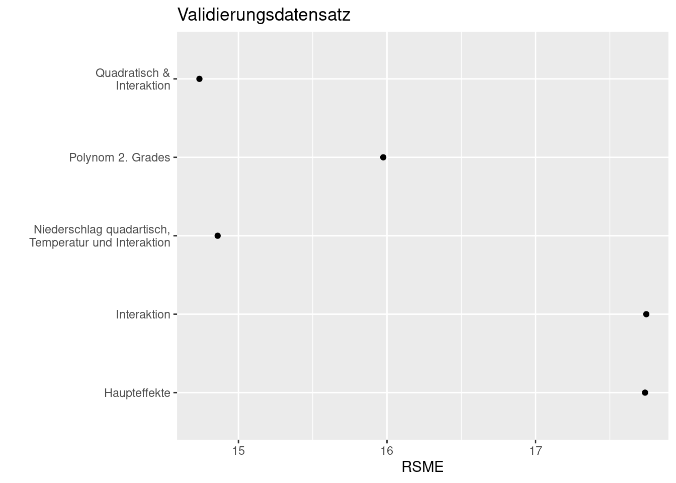

Beim Vergleich mit den Testdaten erkennen wir, dass das Modell mit quadratischem Term bei Niederschlag, dem Haupteffekt für Temperatur und Interaktionen am besten abschneide. Wir sehen hier auch, dass dieses Modell mit der Interaktion und dem quadratischem Effekt deutlich besser generalisiert als das quadratische Modell ohne Interaktionen- beim Trainingsdatensatz sind beide Modelle gleich gut. Der Fehler von 13.5% Waldbedeckung ist allerdings erheblich.

ggplot(data= res, mapping = aes(x= model, y= rsmeTrain)) +
  geom_point() +
  coord_flip() + ylab("RSME") + xlab("") +
  labs(title = "Trainingsdatensatz")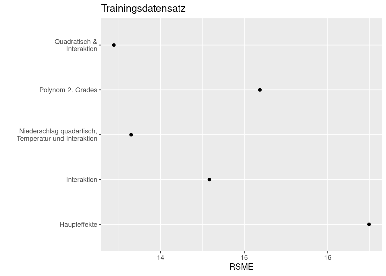

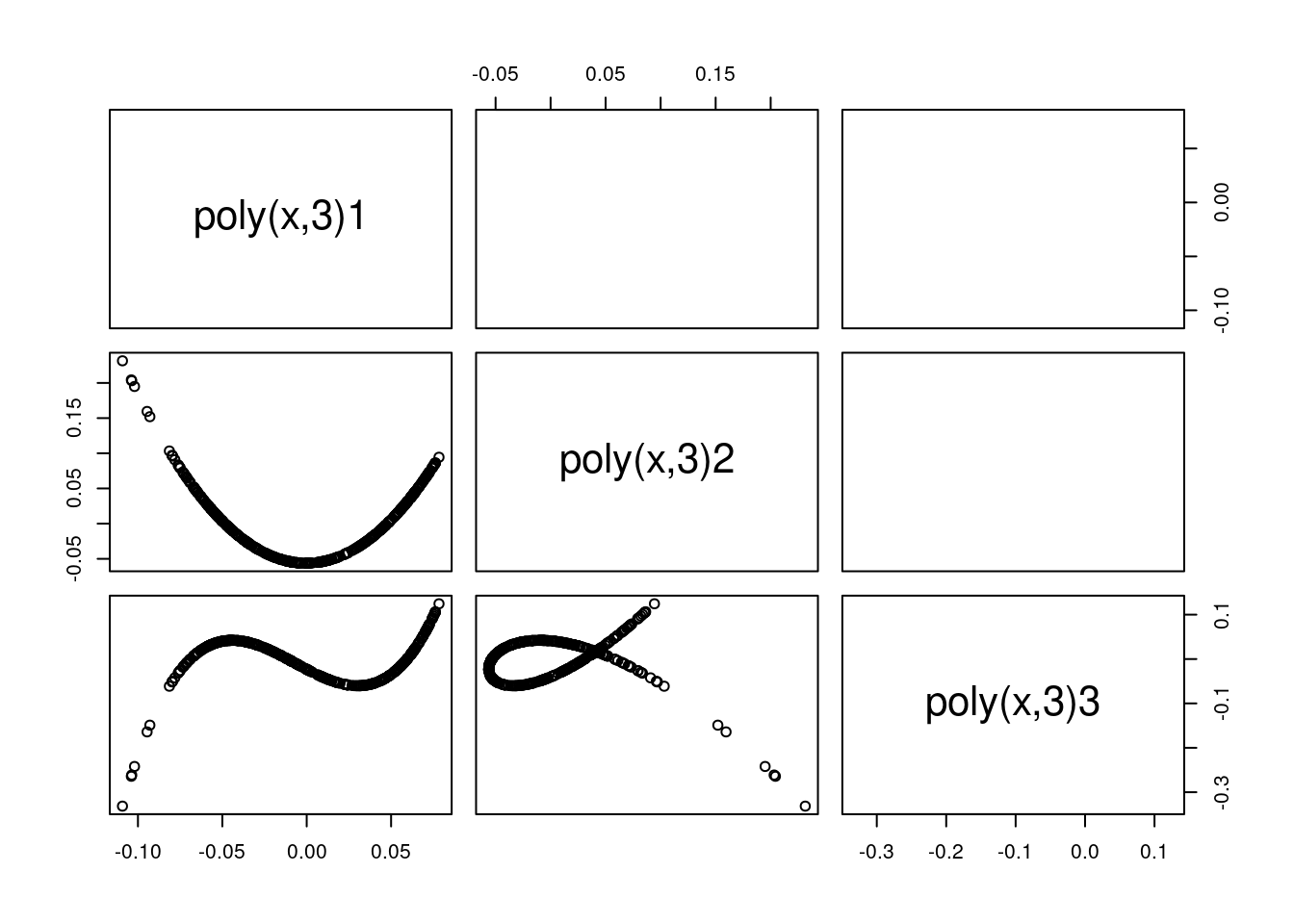
15.5 Exkurs: was passiert bei poly?

bio1.poly3 <- poly(dat.glc2_train$BIO1,3)

Poly erzeugt voneinander unabhängige (orthogonale) Variablen - die Korrelationskoeffizienten sind quasi 0.

pairs(bio1.poly3 , upper.panel = panel.cor, labels=c("poly(x,3)1", "poly(x,3)2", "poly(x,3)3"))

Im Gegensatz dazu sind x, \(x^2\) und \(x^3\) hochgradig korreliert.

pairs(cbind(dat.glc2_train$BIO1, dat.glc2_train$BIO1^2,  dat.glc2_train$BIO1^3 ), upper.panel = panel.cor, labels=c( "x", "x^2", "x^3"))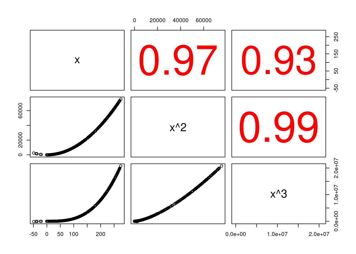

Das erste orthogonale Polygon ist dabei (muss!) perfekt mit x korreliert.

pairs(cbind(bio1.poly3, dat.glc2_train$BIO1, dat.glc2_train$BIO1^2,  dat.glc2_train$BIO1^3 ), upper.panel = panel.cor, labels=c("poly(x,3)1", "poly(x,3)2", "poly(x,3)3", "x", "x^2", "x^3"))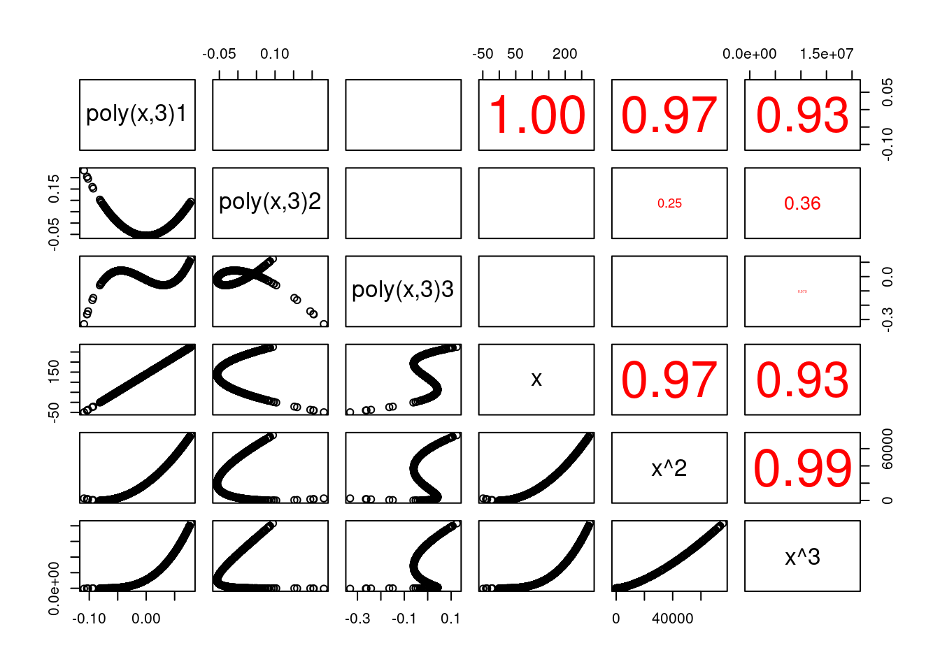

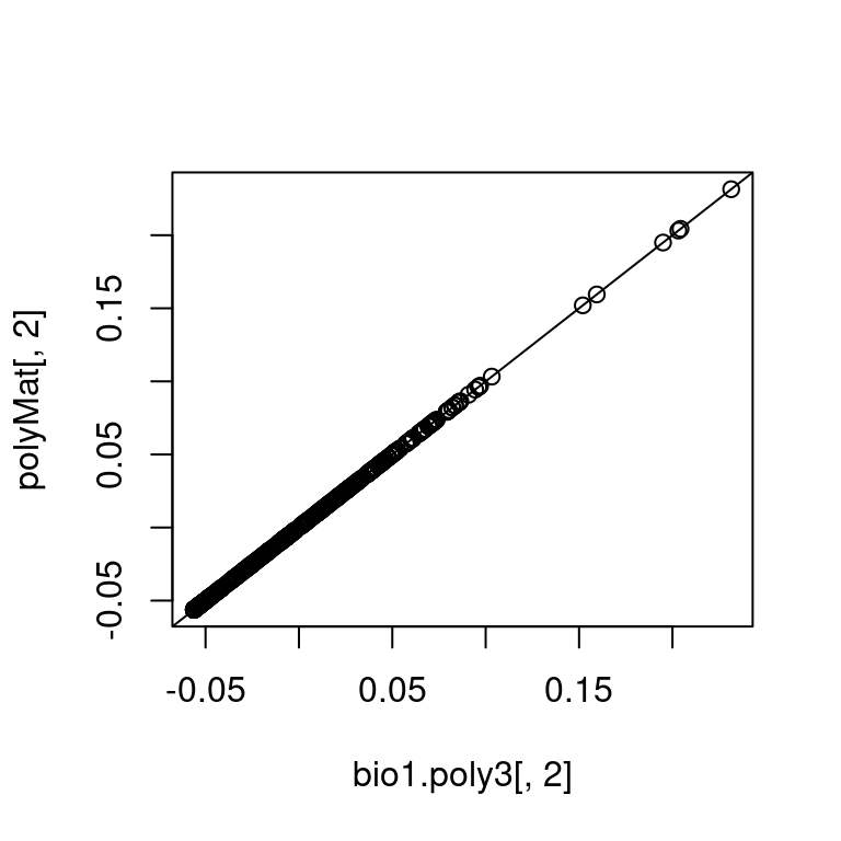
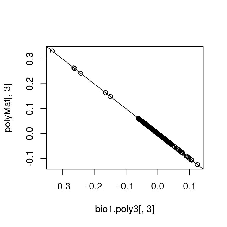
Erzeugen kann man die othronomalen Polygone als QR Zerlegung einer Matrix, die in jeder Spalte \(x^{spaltennummer}\) enthält, die anschließend zentriert wird.

# Matrix mit x, x^2, x^3
polyMat <- cbind(dat.glc2_train$BIO1, dat.glc2_train$BIO1^2, dat.glc2_train$BIO1^3)
# zentrieren
polyMat[,1] <- polyMat[,1] - mean(polyMat[,1])
polyMat[,2] <- polyMat[,2] - mean(polyMat[,2])
polyMat[,3] <- polyMat[,3] - mean(polyMat[,3])
# QR Zerlegung der Matiry
polyMat <- qr.Q(qr(polyMat))

Die so gewonnenen Ergebnisse sind bis auf Rundungsfehler exakt dieselben wie die von poly berechneten.

zapsmall(cor(polyMat,poly(dat.glc2_train$BIO1,3)))

##      1 2  3
## [1,] 1 0  0
## [2,] 0 1  0
## [3,] 0 0 -1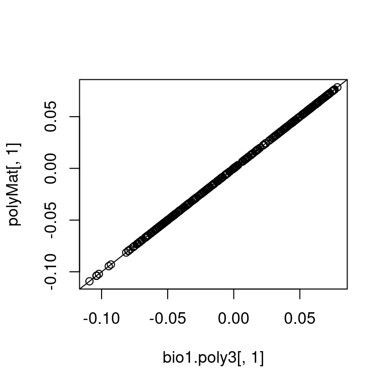

plot(polyMat[,1] ~ bio1.poly3[,1])
abline(lm(polyMat[,1] ~ bio1.poly3[,1]))

plot(polyMat[,2] ~ bio1.poly3[,2])
abline(lm(polyMat[,2] ~ bio1.poly3[,2]))

plot(polyMat[,3] ~ bio1.poly3[,3])
abline(lm(polyMat[,3] ~ bio1.poly3[,3]))

Weiterführende/zitierte Literatur

Anadón, José D, Osvaldo E Sala, and Fernando T Maestre. 2014. “Climate Change Will Increase Savannas at the Expense of Forests and Treeless Vegetation in Tropical and Subtropical Americas.” Journal of Ecology 102 (6): 1363–73.

Thoning, K. W., A. M. Crotwell, and J. W. Mund. 2020. “Atmospheric Carbon Dioxide Dry Air Mole Fractions from Continuous Measurements at Mauna Loa, Hawaii, Barrow, Alaska, American Samoa and South Pole. 1973-2019, Version 2020-08 National Oceanic and Atmospheric Administration (NOAA), Global Monitoring Laboratory (GML), Boulder, Colorado, USA.” https://doi.org/10.15138/yaf1-bk21.

Eine Gerade ist ein Polynom ersten Grades.↩︎
In einem bestimmten Bereich, zu heiß ist auch nichts, quadratischer Effekt.↩︎
Auch hier wieder abhängig vom Pflanzentyp und innerhalb einer ökologischen Nische, die z.B. für Wasserlinien anders aussieht als für Kakteen.↩︎
Die original Daten sind unter folgendem Link abrufbar: [ftp://aftp.cmdl.noaa.gov/data/greenhouse_gases/co2/in-situ/surface/] ↩︎