Kapitel 2 Arbeiten mit R und RStudio
R ist eine Programmiersprache, in der Kommandos zum einlesen der Daten, zum erzeugen von Grafiken und zum berchnen von Statistiken, aber auch für Programmstrukturen wie Schleifen, Funktionen oder Klassen eingegeben werden. Rstudio ist eine IDE (Integrated Development Interface), also eine Arbeitsumgebung, die auf R aufsetzt und das Arbeiten mit R in vielerlei Hinsicht vereinfacht. In diesem Kapitel geht es darum, wie man beide Programme installiert, und wie man grundlegende Arbeitsschritte durchführt. Dazu gehört auch ein kurzer Überblick über die Arbeitsweise in RStudio.
2.1 Setting up R & RStudio
R und RStudio stehen für MS Windows, Mac OS, gebräuchliche Linuxvarianten (ubuntu, debian, fedora, suse, redhat) als binär Dateien zur Installation bereit. Für andere Plattformen, muss die Software aus dem Quellcode kompiliert werden. Mit dem Einsatz auf Samrtphones oder Tablets liegen mir keine Erfahrungswerte vor. Meine Empfehlung ist es auf einem Laptop oder Desktop Rechner zu arbeiten, ggf. im PC-Pool.
Wichtig ist, dass zuerst R installiert wird, dann RStudio.
Falls eine ältere Version von R oder RStudio bereits installiert sein sollte, würde ich empfehlen diese zu aktualisieren. Es ist nicht notwendig, die allerneuste Version zu installieren. Die LTS Version von ubuntu Linux verwendet z.B. i.d.R. eine etwas ältere Version von R. Dies ist unkritisch.
RStudio wird in verschiedenen Versionen vertrieben. Die freie Variante bietet alles, was wir im Kurs (und wahrscheinlich auch im weiteren Berufsleben) benötigen.
2.2 R packages
Der Funktionsumfang von R lässt sich durch Zusatzpakete (packages) erweitern. Diese lassen sich über die Kommandozeile oder über das GUI installieren.
Der nachfolgende Code-Chunk kann dazu genutzt werden, die im Kurs benötigten Pakete zu installieren - dies muss nur einmal passieren. Am einfachsten geht diese, indem man den Code-Chunk kopiert und in die R-Console einfügt (s. weiter unten). Der Code überprüft, ob die Pakete schon installiert sind und installiert fehlende Pakete. Sie werden vermutlich gefragt, von wo Sie die Pakete runterladen möchten. Wählen Sie CRAN.
Achten Sie auf Fehlermeldungen während der Installation. Mitunter fehlen externe Bibliotheken, die separat installiert werden müssen. Üblicherweise sollten aber keine Probleme auftauchen.
thePackages <- c("knitr", "tidyverse", "dplyr", "ggplot2", "sf", "s2", "raster", "terra",
               "tmap",  "GGally", "corrplot", "ggpubr", "ggExtra", "fitdistrplus", "moments",
               "FAdist", "crch", "ggpmisc", "AICcmodavg", "polycor",
               "AMR", "DescTools", "ellipse")
install.packages(setdiff(thePackages, rownames(installed.packages())))
2.3 RStudio interface
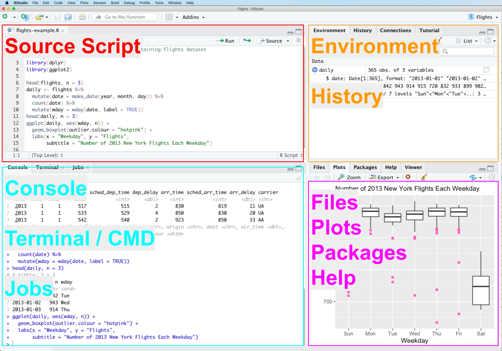
Figure 2.1: RStudio Interface
Source / Script
Der Source Bereich in der linken oberen Ecke enthält den R source code, d.h. die Kommandos die ausgeführt werden sollen. Die Kommandos werden top-down ausgeführt, d.h. oben stehende Kommandos zuerst. Die Reihenfolge ist also wichtig. ZUerst müssen die Daten eingelesen werden, bevor sie geplottet werden können. Mit dem run button oben rechts kann man entweder:
* das ganze Script ausführen
* eine einzelne Zeile ausführen - hierfür muss sich der Cursor in der auszuführenden Zeile befinden. Dann run drücken oder [ctrl] + [enter] drücken. (Die Zeile muss nicht selektiert werden, es reicht, wenn sich der Cursor in der Zeile befindet.)
* mehrere Zeilen oder einen Teil einer Zeile ausführen: hierfür den auszuführenden Bereich selektieren und dann run drücken oder [ctrl] + [enter].
Console
In der Konsole (Console) werden die Befehle ausgeführt. Die Kommandos werden an die Konsole geschickt und dann ausgeführt. Hier erscheinen dann auch Rückmeldungen wie z.B. Fehlermeldungen oder Ergebnisse.
In einem weiteren Reiter befindet sich das Terminal. Hiermit lassen sich Kommandos an das Betriebssystem schicken - je nach Betriebssystem unterscheidet sich das Terminal. Der Bckground Jobs Reiter listet alle R Operationen im HIntergrund auf, wie z.B. ausgeführte Scripte, die unabhängig im Hintergrund laufen. Hierzu zählen z.B. die Installation von paclages. Im RenderReiter werden Jobs ausgeführt, die Knit oder bookdown Befhle umfassen, die also aus RMarkdown Dokumenten HTML, Libre/Microsof Offic Dokumente oder PDF erzeugen.
Environment / History
Das Environment Panel oben rechts listet alle Variablen und Funktionen auf, die im aktuellem Projekt definiert sind. Einzelne Variablen lassen sich anklicken um mehr Informationen zu erhalten - data.frames werden dann angezeigt. Der History Reiter listet alle ausgeführten Kommandos der aktuellen Projektsitzung auf.
Files/Plots/Packages/Help
Das panel unten rechts besteht aus den folgenden Reitern:
* Files: ein Datei Explorer um z.B. neue Ordner anzulegen, Datein zu verschieben, umzubenennen oder zu kopieren. Für manche Dateiformate wie .csv oder .xlsx gibt es ein graphisches Interface, das beim Import behilflich sein kann.
* Plots: alle in der aktuellen Sitzung erzeugten Plots können hier angeschaut werden.
* Packages: zeigt welche packages lokal installiert sind und erlaubt es weitere packages zu installieren. Zeigt auch an ob Updates verfügbar sind.
* Help: Dokumentation der installierten packages. Man kann hier Kommandonamen eintippen. Alternativ kann man Hilfe für einen Befehl auch über ? erhalten, wenn man unmittelbar nach dem Fragezeichen den Befehlsnamen eingibt, z.B. ?read.csv()
2.4 Dateipfadangaben und Projekte in RStudio
In den allermeisten Fällen umfasst das Arbeiten mit R das Arbeiten mit Daten, welche in den Arbeitsspeicher von R geladen werden müssen. Um die Daten laden zu können, müssen wir R sagen, wo sich die Daten befinden. Oftmals handelt es sich um Daten, die in Dateien (Textdateien, OpenOffice Calc oder Microsoft Excel Spread Sheets, dbase-Dateien, Shapefiles, Geopackages, GeoTiffs und vieles mehr) gespeichert sind.1 Wichtig ist dabei, dass wir den Speicherort angeben. Ebenso ist es möglich, Daten aus R heraus zu exportieren, wofür ebenfalls neben dem Dateinamen der Speicherort angegeben werden muss. Weiterhin sollen Script Dateien und RMarkdown Dateien, in denen wir Kommandos speichern irgendwo im Dateisystem gespeichert werden. In all diesen Fällen benötigen wir neben dem Dateinamen noch einen Dateipfad, der angibt, wo auf unserer Festplatte oder auf einem Netzlaufwerk die Datei zu finden ist bzw. angelegt werden soll.
Pfadangaben können dabei absolut oder relativ gemacht werden. Absolute Pfadangaben beziehen sich auf das Wurzelverzeichnis des Laufwerks, während relative Pfade relativ zu einem Verzeichnis angegeben werden. Beispiele für absolute Pfadangaben sind z.B.:
C:\meinNutzerName\Eigene Dateien\Studium\Geographie\Einführung_Statistik\(Microsoft Windows)N:\arbeitsgruppeGIS\OSManalysen\completeness\jakarta\(Microsoft Windows)/meinNutzerName/home/Documents/Studium/Geographie/EInfuehrung_Statistik/(Linux oder MacOS)
Relative Pfadangaben werden ausgehend von einem Ausgangsverzeichnis definiert, z.B.:
- “im gleichen Verzeichnis”
- “steige im gleichen Verzeichnis in der Ordner XYZ ab”
- “steige zwei Verzeichnisse nach oben und dann in den Ordner ABC ab”
- “Im Wurzelverzeichnis des Servers giscience.courses-pages.gistools.geog.uni-heidelberg.de steige in den Ordner einfuerung_statistik ab”
Dabei gibt es ein relevantes Sonderzeichen: ../ was soviel heißt wie “steige ein Verzeichnis auf”.
Relative Pfadangaben haben verschiedene Vorteile. So sind sie oft kürzer. Wenn Sie sich schon im Verzeichnis XY befinden und dort eine Datei “Pisa.csv” finden, muss ich Ihnen nicht langwierig erklären, wie Sie zu diesem Verzeichnis gelangen, sondern Sie können die Datei einfach laden.2 Daneben lassen sich darüber Angaben über verschiedene Umgebungen vereinheitlichen. So unterscheiden sich die Speicherorte für das Verzeichnis zur Statistik-Übung vermutlich sehr stark: der eine arbeitet unter einem deutschen Windows 11 System, die andere unter ubuntu Linux, eine Erasmusstudierende auf einem französischem MacOS, ein Studierender gruppiert seine Dateien nach Studiengängen und Semestern, ein anderer Strukturiert nur nach den Veranstaltungen, noch ein weiterer differenziert noch eninmal zwischen Vorlesung und Übung,… Falls ich jeden von Ihnen erklären sollte, welche Datei Sie laden sollen, wäre dies problematisch, wenn ich dies über absolute Pfadangaben vornehmen wollte. Einfacher geht es wie folgt: Wenn Sie sich alle an generelle Anweisungen halten (“Legen Sie an einem beliebigem Ort einen Ordner ‘Statistik’ an und darin einen Unterordner”Uebung_1”, kopieren alle Dateien die Daten enthalten in einen weiteren Unterordner ‘daten’ in “Uebung_1” und setzen Sie ’Uebung_1” als Arbeitsverzeichnis), dann kann ich Ihnen einfach sagen “Laden Sie die Datei ‘daten/Pisa.csv’”.
Lassen Sie uns noch einmal einen Beispielordner anschauen3:
spatial_data_science/
├── notes.docx
├── spatial_data_science.Rproj
├── data
│   ├── acled_example.xlsx
│   ├── covid19_incidence_kreise.xlsx
│   ├── meuse.dbf
│   └── osm_bw.gpkg
└── src
    ├── exercise_1.Rmd
    ├── exercise_2.Rmd
    └── exercise_3.Rmd
Absolute Pfadangaben erfolgen wie gesagt relativ zum Wurzelverzeichnis ihres lokalen Dateisystems. Unter einem Windows Betriebssystem z.B.:
c:/Documents and users/Desktop/Uni_stuff/classes/spatial_data_science/data/covid19_incidence_kreise.xlsx
Relative Pfadangaben erfolgen relativ zum Arbeitsverzeichnis eines Programme (hier R). Wenn R mit folgendem Arbeitsverzeichnis arbeitet:
c:/Documents and users/Desktop/Uni_stuff/classes/spatial_data_science/src/
Dann kann man den relativen Pfad zum covid19 Datensatz so angeben:
../data/covid19_incidence_kreise.xlsx
“../” heißt soviel wie “steige ein Verzeichnis auf”.
Hinweis: Windows verwendet den Backslash * für Pfadangaben. Dies funktioniert nicht mit R. Anstelle dessen muss der Slash /* oder ein doppelter Backslash \ verwendet werden.
c:/Documents and users/Desktop/Uni_stuff/classes/spatial_data_science/data/covid19_incidence_kreise.xlsxfunktioniertc:\Documents and users\Desktop\Uni_stuff\classes\spatial_data_science\data\covid19_incidence_kreise.xlsxfunktioniert nichtc:\\Documents and users\\Desktop\\Uni_stuff\\classes\\spatial_data_science\\data\\covid19_incidence_kreise.xlsxfunktioniert.
Um das aktuelle Arbeitsverzeichnis herauszufindenfunktioniert verwendet man getwd(). Um das Arbeitsverzeichnis zu ändern (z.B. auf /home/fl789/documents/uni/classes/sds/) kann man setwd("/home/fl789/documents/uni/classes/sds/") verwenden. Es ist jedoch nicht empfohlen, die Pfade hard im Script zu setzen. Der empfohlene Weg ist es, über RStudio-Projekte (.Rproj Dateien) das Arbeitsverzeichnis zu setzen. Man legt ein neues Projekt an, wählt das relevante Verzeichnis aus (in unserem Beispiel c:/Documents and users/Desktop/Uni_stuff/classes/spatial_data_science/), fertig. Von da an werden alle Pfade relativ zu diesem Verzeichnis interpretiert.
Das folgende animierte .gif zeigt, wie man ein neues R-Projekt anlegt:
Figure 2.2: Wie legt man ein neues R project in RStudio an.
2.5 Rmarkdown
Für die Übungen nutzen wir R Markdown Dateien.4 R Markdown Dateien kombinieren klassischen Markdown Text, R code mit Ergebnissen der R-Funktionen wie Text, Abbildungen oder Animationen. R Markdown Dateien können über die knit Funktion (oder das RStudio Menu) in pdf, docx und html Dateien kompiliert werden.
Mehr Informationen zur R Markdown Syntax findet sich hier: https://rmarkdown.rstudio.com/lesson-1.html.
Ein Überblick zur Markdown Syntax findet sich hier: https://www.markdownguide.org/basic-syntax/
Figure 2.3: R Markdown Source file, knitting and result in html
Die generelle Struktur einer RMarkdown Datei sieht wie folgt aus:
- ein YAML5 Header mit Meta-informationen wie dem Autor, dem Title, dem Datum, dem Ausgabeformat und vielem mehr
- code chunks, welche den ausführbaren R-code enthalten
- normaler Text (z.B. Notizen, Erklärungen), der mithilfe der Markdown Sprache formatiert werden kann
- zusätzlich können LaTeX Formeln eingebunden werden, LaTeX Kommandos direkt eingebunden werden und vieles mehr, was aber hier zu weit führt.
2.6 Weiterführende Ressourcen
Wie können Sie sich selbst weiterhelfen, wenn es einmal klemmt?
Schauen Sie in die Hilfe zur jeweiligen Funktion - erreichbar mittels
?<function name>innerhlab von RStudio, über den Help Reiter oder auch über F1 zu einem markierten FunktionsnamenLesen Sie die vignettes des jeweiligem pacckages, das Sie benutzen wollen. Eine Vignette ist eine ausführliche Anleitung, welchem Zweck ein package dient und wie die wichtigsten Funktionen funktionieren. Bevor Sie eine Suchmaschine oder einen chatbot befragen, werfen Sie doch einmal einen Blick in die entsprechende Vignette.
Google it.6 R ist eine sehr populäre Software mit einer großen Community. Die meisten Probleme denen Sie begegnen wurden bereits online diskutiert. Formulieren SIe Ihre Frage am besten auf English. Versuchen Sie die richtigen Begriffe zu verwenden, z.B. :
R how to join two tables based on multiple columns?
Vermutlich führt Sie die Suchmaschine zu Stackexchange oder Stackoverflow.
Daneben lassen sich natürlich auch chatbots nutzen. Wenn es nicht um weitergehende Erklärungen geht sollte man allerdings den Ressourcenverbrauch bedenken, der deutlich höher ist als gemeinhin angenommen. Auch Google liefert neuerdings auch stets eine KI generierte Zusammenfassung mit - alternative Suchmaschinen verzichten - noch - darauf. Des weiteren sollte man sich klar machen, dass die den chatbots zugrunde liegenden LLMs kein Verständnis der Zusammenhänge haben sondern nur Wörter aufgrund gelernter Wahrscheinlichkeiten zusammenfügen. Das klappt oftmals überraschend gut, liegt mitunter aber auch dramatisch daneben.
- Cheatsheets sind in der R Community sehr populär. Beispiele sind:
- Bücher und Online Ressourcen
Viele der genannten Bücher sind in der Universitätsbibilothek Heidelberg als Druckversion oder teilweise auch als Onlineressource verfügbar.
- (Carsten F. Dormann 2013): Sehr gute Einführung in die parametrische Statistik anhand von R mit Beispielen aus der Ökologie.
- Eine Vorläuferversion des Buches findet sich sich auf den Seiten von CRAN unter Contributed Documentation
- (Field, Miles, and Field 2012): Locker geschriebene Übersicht über Statistik mit R. Englisch.
- (Gotelli and Ellison 2004): Gute Methodenübersicht, allerdings ohne Beispiele in R oder einer andern Statisiksoftware. Anwendungsbeispiele aus der Ökologie. Englisch.
- (Hedderich and Sachs 2018): Umfangreiches Übersichtswerk das neben Theorie auch Beispiele in R enthält.
- (Jones, Harden, and Crawley 2022): Umfangreiches Werk zur Einführung in die Statistik anhand von R und in das Arbeiten mit R. Anwendungsbeispiele aus der Ökologie.
- (Faraway 2004) und (Faraway 2016): Einführung und fortgeschrittene Regressionsverfahren. Alle Anwendungen in R. Breites Spektrum von Beispielen aus diversen Anwendungsdisziplinien. Englisch.
- Eine Vorläuferversion der Bücher findet sich sich auf den Seiten von CRAN unter Contributed Documentation
- eine Vielzahl von Manuals in verschiedenen Sprachen findet sich auf den Seiten von CRAN unter Contributed Documentation
- (Dunn and Smyth 2018): für Fortgeschrittene, bietet neben dem linearen Modell eine sehr gute Darstellung des generalisierten linearen Modells; zahlreiche Anwendungsbeipiele und Aufgaben mit R
Weiterführende/zitierte Literatur
Daneben können auch Verbindungen zu Datenbanken wie PostgreSQL, Oracle, oder Mongo-DB hergestellt werden um darin gespeicherte Daten zu laden.↩︎
Eine Analogie sind Wegbeschreibungen: stellen Sie sich vor, Sie befinden sich bereits im Gebäude INF 348 in Heidelberg in Baden-Württemberg und fragen nach dem Weg zum Sekretariat der GIScience Gruppe. Wäre es dann nicht einfacher, den Weg relativ zum aktuellem Ort, z.B. Seminarraum 015 zu erklären “ein Stockwerk hoch, dann rechts, den Gang entlang bis zum Büro XX”, als den Weg von einem weit entfernten Referenzpunkt (z.B. Koordinatenursprung 0° nördlicher Breite, 0° westlicher Länge, Reichstag in Berlin, Bismarckpaltz in Heidelberg) zu erklären?↩︎
Ordner und Verzeichnis benutze ich als Synonym.↩︎
Das Kursbuch ist mit einer Erweiterung bookdown geschrieben.↩︎
Oder eine andere Suchmaschine wir DuckDuckGo.↩︎