Chapter 4 Spatial Data
R and RStudio can be used as a code based GIS. Base R and the tidyverse packages already provide a wealth of functionality for traditional non-spatial data science. This is complemented by packages on spatial data processing and visualization packages.
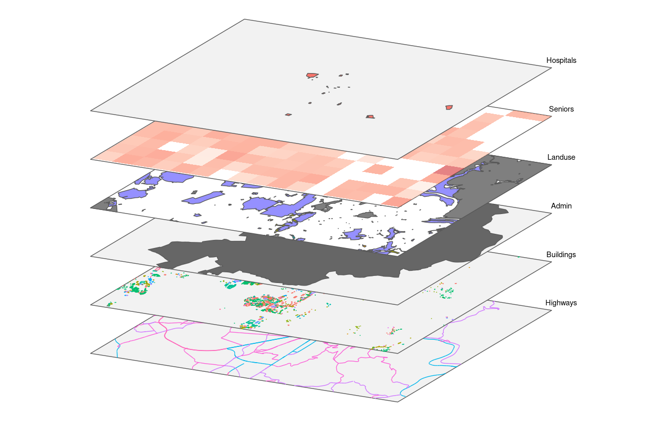
(#fig:R_as_GIS)GIS Layer principle
Datasets used in this example
ACLED
The dataset was already used in @ref(non-spatial_data). Refer to the chapter for further details.
The dataset can be downloaded as .xlsx here
Weekly COVID incidence rates on the Kreis / district level
The dataset is preprocessed. It contains the covid incidence numbers, the Kreis/district geometries and some additional socioeconomic variables.
Here is a list of the sources:
- RKI COVID 19 daily reportings: https://www.arcgis.com/home/item.html?id=f10774f1c63e40168479a1feb6c7ca74
- Kreis Grenzen: https://gdz.bkg.bund.de/index.php/default/verwaltungsgebiete-1-250-000-mit-einwohnerzahlen-ebenen-stand-31-12-vg250-ew-ebenen-31-12.html
- INKAR Socio-economic indicators: https://www.inkar.de/
The dataset can be downloaded as .gpkg here
4.1 R Libraries for spatial data
R packages for handling spatial data:
Vector data
sp1st gen spatial data librarysf2nd gen spatial data library - closer to data frame structure, more convenient, implements base dplyr/tidy methods
Raster data
raster1st gen raster libraryterra2nd gen raster library (a whole lot faster)stars2n gen raster library. Emphasis on spatio-temporal use cases. Combination of raster and vector to data cubes. Proxy stars objects provide a solution to bigger than memory raster files .
These packages are only de facto standard packages for reading, writing, and simple processing of spatial data. Many packages with more specialized use cases, such as spatial modeling or network analysis, are built on top of these packages. But not all of these packages support all available types of spatial data structures in R. Therefore it may be necessary to convert the object from one type to another for some functions.
The story behind a package can vary greatly. Some are developed and maintained by just one or a few people. Others by institutes or companies. Sustainability is a particular challenge here. As users we should always look at how old a package is, is it still maintained, are there possibly other packages that continue the functionality. Every package on CRAN has a release date. Many packages are hosted on github and the development can be observed quasi publicly. There you can also check what the last version of a package is and when it was released.
Conversion between vector structures:
Conversion between raster structures:
4.2 Vector data
What dplyr is for tabular data structures in R, is sf for vector data structures.
All common spatial operations are implemented. You can easily implement workflows from QGIS, ArcGIS or PostGIS.
At the same time sf is very close to the data.frame class of R and you can apply non-spatial operations on features and their attributes.
The following schema shows the location of the sf package between other R packages and external, standard geoinformatics software packages. Notably GDAL, GEOS and PROJ are well-known external libraries used by QGIS and PostGIS among others.
Important: When sf is called in a R session for the first time, it will print the versions of the linked external libraries. This can be important because some functions in newer versions may contain new parameters or their functionality may change. This happened for example with GEOS 3.8. Since this version it is possible to set a tolerance parameter for every geometric operation. The parameter allows for reducing the amount of digits in coordinates of a geometry.
## Linking to GEOS 3.12.1, GDAL 3.8.4, PROJ 9.4.0; sf_use_s2() is TRUE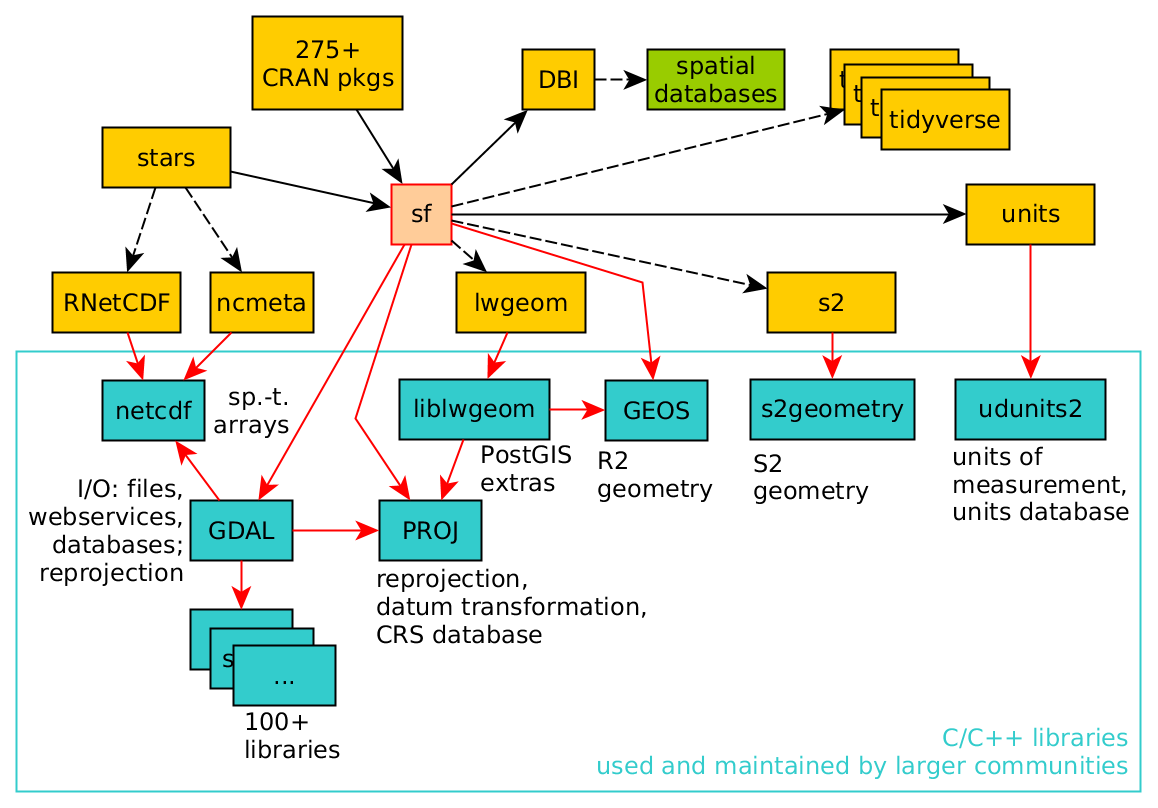
(#fig:sf deps)sf and its dependencies; arrrows indicate strong dependency, dashed arrows weak dependency (source: Edzer et al. 2022)
The following shows an example sf dataframe structure. As mentioned, it is very close base R’s data frames.
Every sf dataframe has header information on geometry type, dimension, its extent or bounding box and its CRS. Also there is a dedicated geometry column.
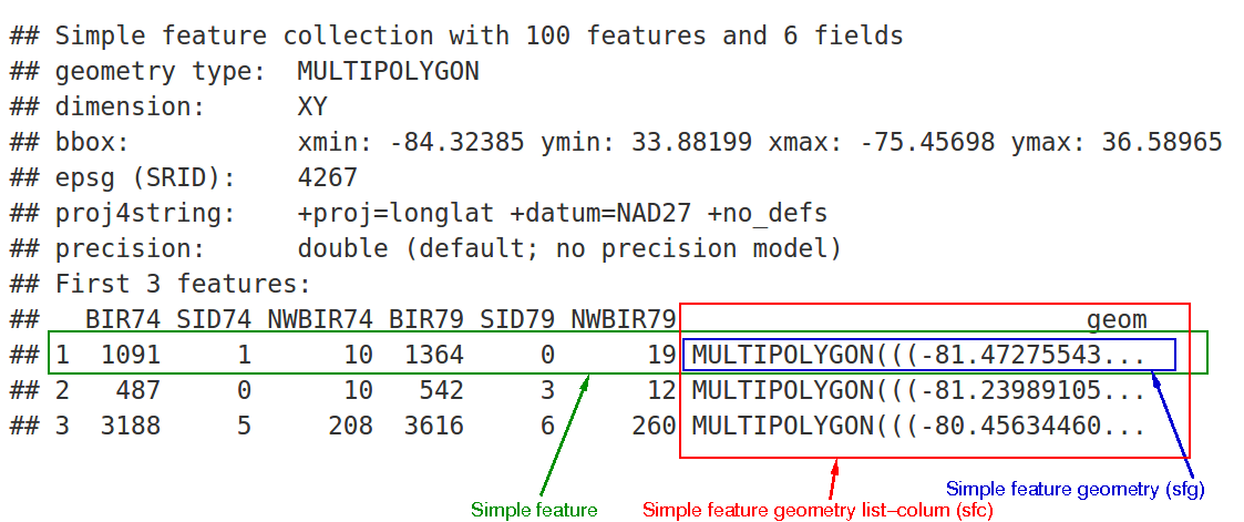
(#fig:sf dataframe)sf and its dependencies; arrrows indicate strong dependency, dashed arrows weak dependency
We use the acled data.frame to understand the sf dataframe structure. The excel file contains a latitude and longitude attributes which we use to build a point geometry and subsequently convert the whole dataframe into a sf dataframe.
##
## Attaching package: 'dplyr'
## The following objects are masked from 'package:stats':
##
## filter, lag## The following objects are masked from 'package:base':
##
## intersect, setdiff, setequal, unionacled_africa <- read_excel("data/Africa_1997-2022_Apr22.xlsx")
# create a subset
acled_africa <- acled_africa |>
filter(YEAR > 2021)
library(sf)
# select the first row to create a single point location
single_row <- acled_africa[1,]
st_point(c(single_row$LONGITUDE, single_row$LATITUDE))## POINT (6.615 36.365)## [1] "XY" "POINT" "sfg"# convert the whole dataframe to a sf dataframe
acled_africa.sf <- st_as_sf(acled_africa, coords = c("LONGITUDE", "LATITUDE"))
acled_africa.sf |> class()## [1] "sf" "tbl_df" "tbl" "data.frame"## [1] "sfc_POINT" "sfc"## Simple feature collection with 6 features and 27 fields
## Geometry type: POINT
## Dimension: XY
## Bounding box: xmin: -0.668 ymin: 35.404 xmax: 8.124 ymax: 36.75
## CRS: NA
## # A tibble: 6 × 28
## ISO EVENT_ID_CNTY EVENT_ID_NO_CNTY EVENT_DATE YEAR TIME_PRECISION
## <dbl> <chr> <dbl> <dttm> <dbl> <dbl>
## 1 12 ALG11974 11974 2022-01-03 00:00:00 2022 1
## 2 12 ALG11975 11975 2022-01-03 00:00:00 2022 1
## 3 12 ALG11976 11976 2022-01-04 00:00:00 2022 1
## 4 12 ALG11981 11981 2022-01-05 00:00:00 2022 2
## 5 12 ALG11980 11980 2022-01-05 00:00:00 2022 1
## 6 12 ALG11977 11977 2022-01-05 00:00:00 2022 1
## # ℹ 22 more variables: EVENT_TYPE <chr>, SUB_EVENT_TYPE <chr>, ACTOR1 <chr>,
## # ASSOC_ACTOR_1 <chr>, INTER1 <dbl>, ACTOR2 <chr>, ASSOC_ACTOR_2 <chr>,
## # INTER2 <dbl>, INTERACTION <dbl>, REGION <chr>, COUNTRY <chr>, ADMIN1 <chr>,
## # ADMIN2 <chr>, ADMIN3 <lgl>, LOCATION <chr>, GEO_PRECISION <dbl>,
## # SOURCE <chr>, SOURCE_SCALE <chr>, NOTES <chr>, FATALITIES <dbl>,
## # TIMESTAMP <dbl>, geometry <POINT>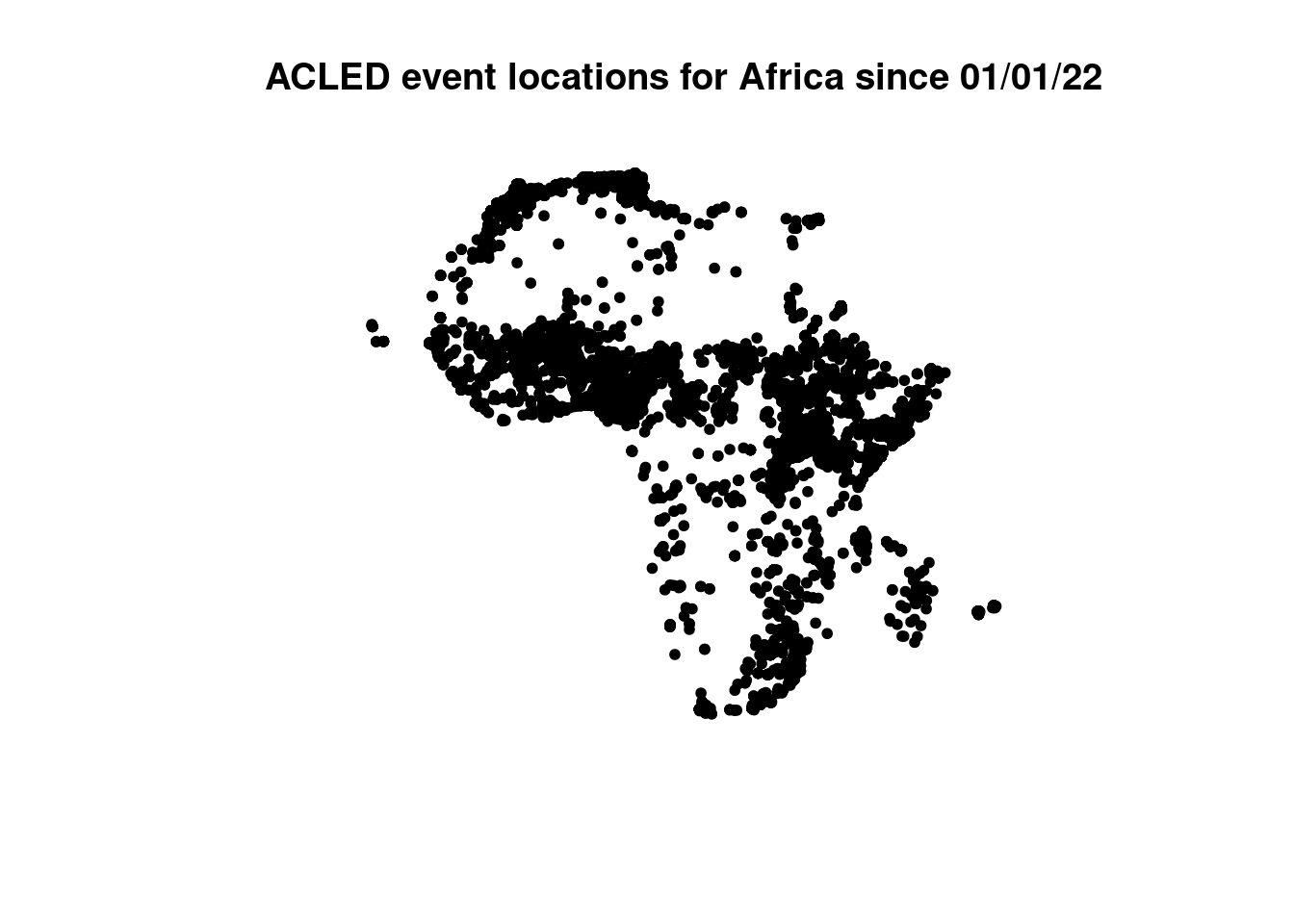
The sf dataframe we created out of ACLED has the geometry type POINT. We did not specify the CRS therefore it is NA. More on CRS and how to assign and reproject in the following sections.
Other geometry types available in sf
The following schema depicts other geometry types available in the simple feature standard. You are probably familiar with these.
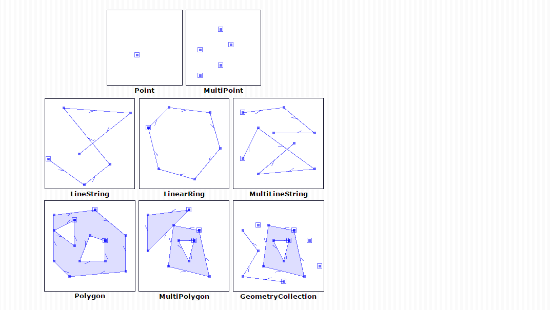
(#fig:simple feature geom types) Simple Feature Model (source: https://autogis-site.readthedocs.io/en/latest/_images/SpatialDataModel.PNG)
The geometry column of a sf data frame is sticky. This means if you manipulate it e.g. in dplyr, the geometry column will always be present in the output. Even if you explicitly deselect it. If you want to get rid of the geometry column, or want to convert your spatial dataframe to a non-spatial one you need to set the geometry NULL:
Another way of dropping the sticky geometry is using st_drop_geometry - see the corresponding help file.
4.2.1 Spatial predicates
All common spatial predicates or relations and geometric operations are available in the sf package. A Selection of predicates:
st_equals()st_touches()st_overlaps()st_contains()st_disjoint()st_covers()st_crosses()
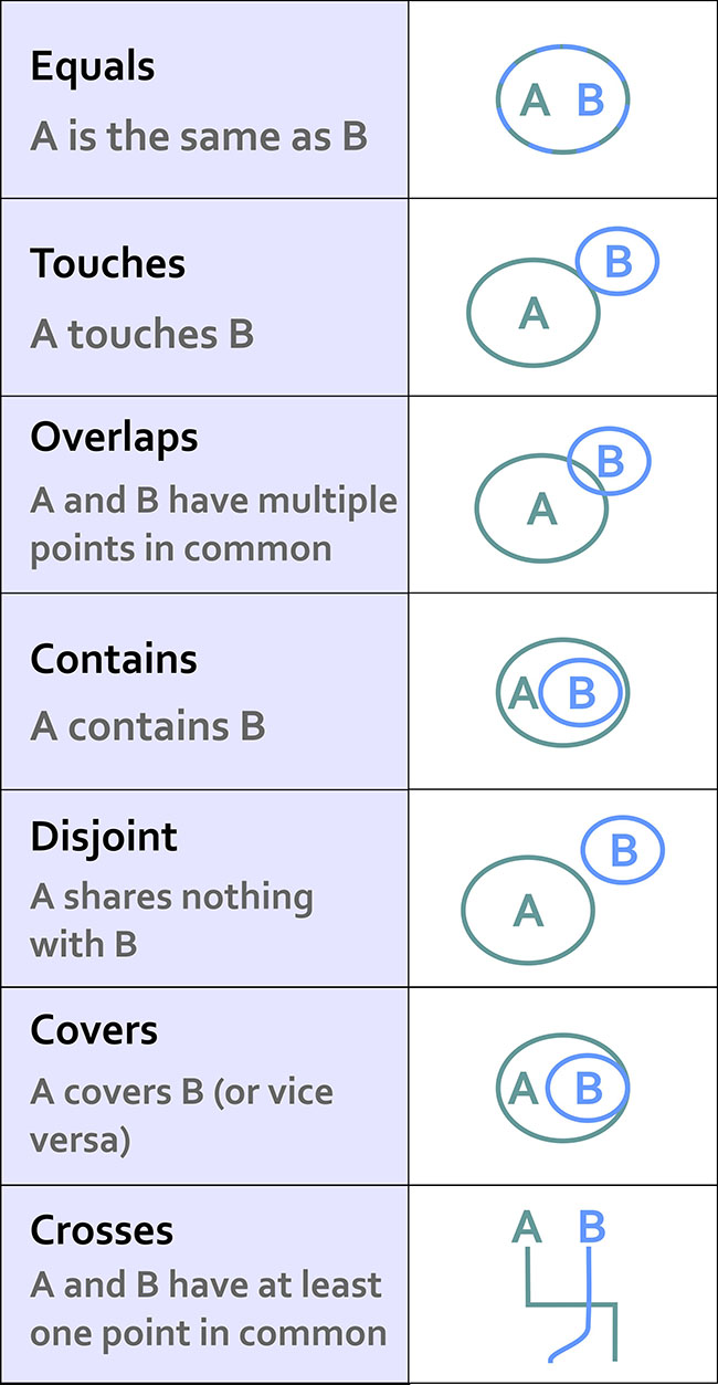
(#fig:spatial predicates)Spatial relationsships (source: https://www.e-education.psu.edu/maps/l2_p5.html)
The standard output format of a spatial predicate in sf is a spatial predicate list. For every feature in dataset A, all features of dataset B for which the predicate is TRUE are listed by Id.
4.2.2 Geometric operations
A Selection of geometric operations:
* st_combine()
* st_union()
* st_intersection()
* st_difference()
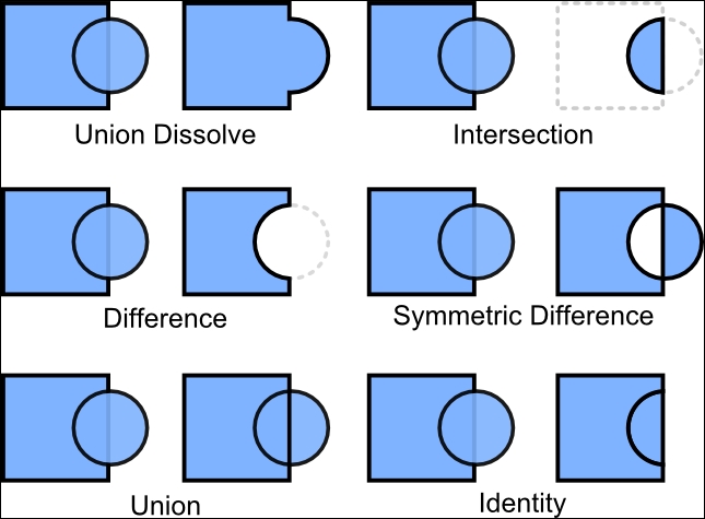
(#fig:geometric operations)Geometric operations (source: https://static.packt-cdn.com/products/9781783555079/graphics/50790OS_06_01.jpg)
4.2.3 CRS and projections
For an example on CRS and projections with sf in R we use country boundary data from geoboundaries.org/. There is a R package available that let us download boundaries for countries within R.
library(rgeoboundaries) # to install, execute: remotes::install_github("wmgeolab/rgeoboundaries")
countries <- gb_adm0() # download all countries
plot(countries$geometry, main="Global boundaries form geoboundaries.org")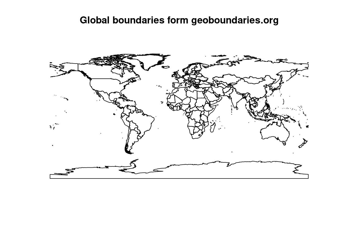
The package is in a kind of experimental stage. It is not published on CRAN and therefore not able to install via the command install.packages("rgeoboundaries"). But it is published on github and can be installed via remotes::install_github("wmgeolab/rgeoboundaries").
The package rgeoboundaries fetches country border data from the geoboundaries website. In the following we use our ACLED dataset to filter for countries that intersect event locations. To achieve this, we need to consider the points below:
- Make sure both datasets share the same CRS. The CRS can be verified and manipualted with the
st_crsfunction. - Create a convex hull for the ACLED event data.
- Use the
st_intersects()function to filter for countries that intersect with convex hull.
## [1] FALSE## Coordinate Reference System:
## User input: WGS 84
## wkt:
## GEOGCRS["WGS 84",
## DATUM["World Geodetic System 1984",
## ELLIPSOID["WGS 84",6378137,298.257223563,
## LENGTHUNIT["metre",1]]],
## PRIMEM["Greenwich",0,
## ANGLEUNIT["degree",0.0174532925199433]],
## CS[ellipsoidal,2],
## AXIS["latitude",north,
## ORDER[1],
## ANGLEUNIT["degree",0.0174532925199433]],
## AXIS["longitude",east,
## ORDER[2],
## ANGLEUNIT["degree",0.0174532925199433]],
## ID["EPSG",4326]]## Coordinate Reference System: NAWe first checked if the CRS of country boundaries and ACLED match. They don’t. ACLED has no CRS set, it’s NA. The countries sf dataframe CRS is EPSG:4326. The Events in ACLED are actually also in EPSG:4326, we can tell from the website’s documentation and when looking at the raw coordinates. We need to assign the CRS to the ACLED sf dataframe:
## [1] TRUEA CRS can be assigned or set by the EPSG code, like in the example above or by pointing to another dataset’s CRS like this:
Important: This not to be to be confused with st_transform(x, crs=) which transforms or reprojects a sf data frame to a different CRS. E.g from EPSG:4326, decimal degrees to EPSG:32632, meters. EPSG:32632 is a projection of the UTM system. It is Zone 32N and covers Germany. The CRS is now set and verified. Next we create the convex hull.
As a rule, we assign a CRS then a geodataset does not contain information about the CRS (and we know it, e.g. because we checked the website, asked the data provider,…). For that operation it is essential that we know the CRS the dataset is in. If we don’t know the CRS and we assign something we might end up in big trouble. Sometimes we have to guess the CRS. In this case we need to carefully check if our guess is correct (e.g. by setting tmap to interactive and checking if the data aligns well with the base map).
If a geodataset has a correct CRS assigned and we want to reproject it to a different CRS we use st_transform which will return a new dataset in the different CRS.
Mixing both things up will cause serious trouble and might ruin all your following analysis steps.
4.2.4 Filtering by spatial predicate
First, all points are combined into a single feature of type multipoint using the command union. Then the function st_convex_hull is executed. a convex hull generates a polygon which encloses all points in the output data set. The vertices of the polygon are determined directly from the location of the outermost points.
## [1] "sfc_POLYGON" "sfc"plot(acled_cv, main="ACLED event locations & convex hull")
plot(acled_africa.sf$geometry, pch=20, add=T)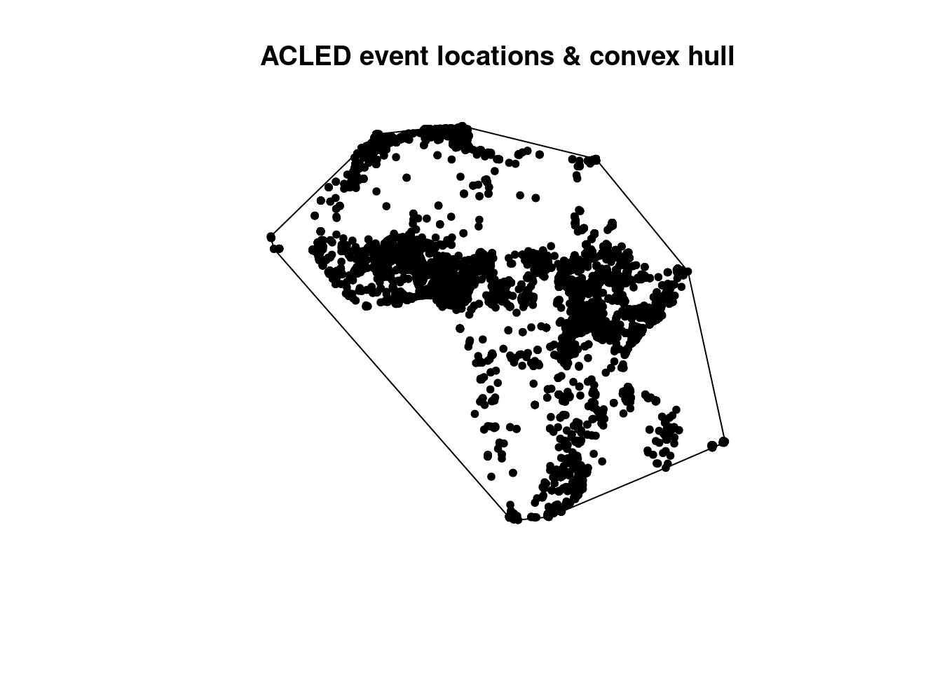
After applying the convex hull function, the geometry type is changed from point to polygon. The simple plot shows the extent of the convex hull and all points are located inside. We called two times the plot function, first for the convex hull, second for the points. The combination of both plots is realized by the parameter add=TRUE in the second plot. This is base R plotting, but especially relevant when you want to combine layers visually.
Next, we use the convex hull to filter all countries that intersect from the global countries dataset.
## Error in wk_handle.wk_wkb(wkb, s2_geography_writer(oriented = oriented, : Loop 92 is not valid: Edge 16120 crosses edge 28118Three geometries have invalid spherical geometries. You can either ignore the issue and go ahead the with the brute force method of deactivating the use of a spherical geometry model in your r session with the following command.
Operations and predicates of sf are then executed on a planar geometry model. This can lead to loss of spatial accuracy if you do not project your data. In essence you will get a lot of warnings when using sf functions on data in EPSG 4326 and s2 turned off.
Therefore we take a closer look at the invalid geometries
## Simple feature collection with 3 features and 1 field
## Geometry type: MULTIPOLYGON
## Dimension:     XY
## Bounding box:  xmin: -180 ymin: -89.99893 xmax: 180 ymax: 81.86122
## Geodetic CRS:  WGS 84
##            shapeName                       geometry
## 1               Fiji MULTIPOLYGON (((-178.7362 -...
## 2 Russian Federation MULTIPOLYGON (((131.8316 42...
## 3         Antarctica MULTIPOLYGON (((-57.02285 -...
countries |>
st_make_valid(geometry) |>
filter(st_is_valid(geometry)==F) |>
dplyr::select(shapeName)## Simple feature collection with 0 features and 1 field
## Bounding box: xmin: NA ymin: NA xmax: NA ymax: NA
## Geodetic CRS: WGS 84
## [1] shapeName geometry
## <0 rows> (or 0-length row.names)We see that Fiji, the russian Federation and Antarctica according to the function st_valid() consist of invalid geometries. Perhaps there is a connection as all these geometries intersect the date line. With the sf function st_makvalid() we can repair the geometries. But use this with caution, this can also lead to technically valid geometries but their shape does not reflect the original phenomenon anymore.
## Sparse geometry binary predicate list of length 198, where the
## predicate was `intersects'
## first 10 elements:
##  1: (empty)
##  2: (empty)
##  3: 1
##  4: 1
##  5: 1
##  6: 1
##  7: 1
##  8: (empty)
##  9: (empty)
## 10: (empty)## [,1]
## [1,] FALSE
## [2,] FALSE
## [3,] TRUE
## [4,] TRUE
## [5,] TRUE
## [6,] TRUEcountries.intersects <- countries |>
filter(st_intersects(geometry, acled_cv, sparse=F)) # setting sparse here is important as dplyr::filter() takes logical statements only## Warning: Using one column matrices in `filter()` was deprecated in dplyr 1.1.0.
## ℹ Please use one dimensional logical vectors instead.
## This warning is displayed once every 8 hours.
## Call `lifecycle::last_lifecycle_warnings()` to see where this warning was
## generated.plot(countries.intersects$geometry, main="Intersecting countries, convex hull & ACLED event locations")
plot(acled_cv, add=T)
plot(acled_africa.sf$geometry, pch=20, add=T)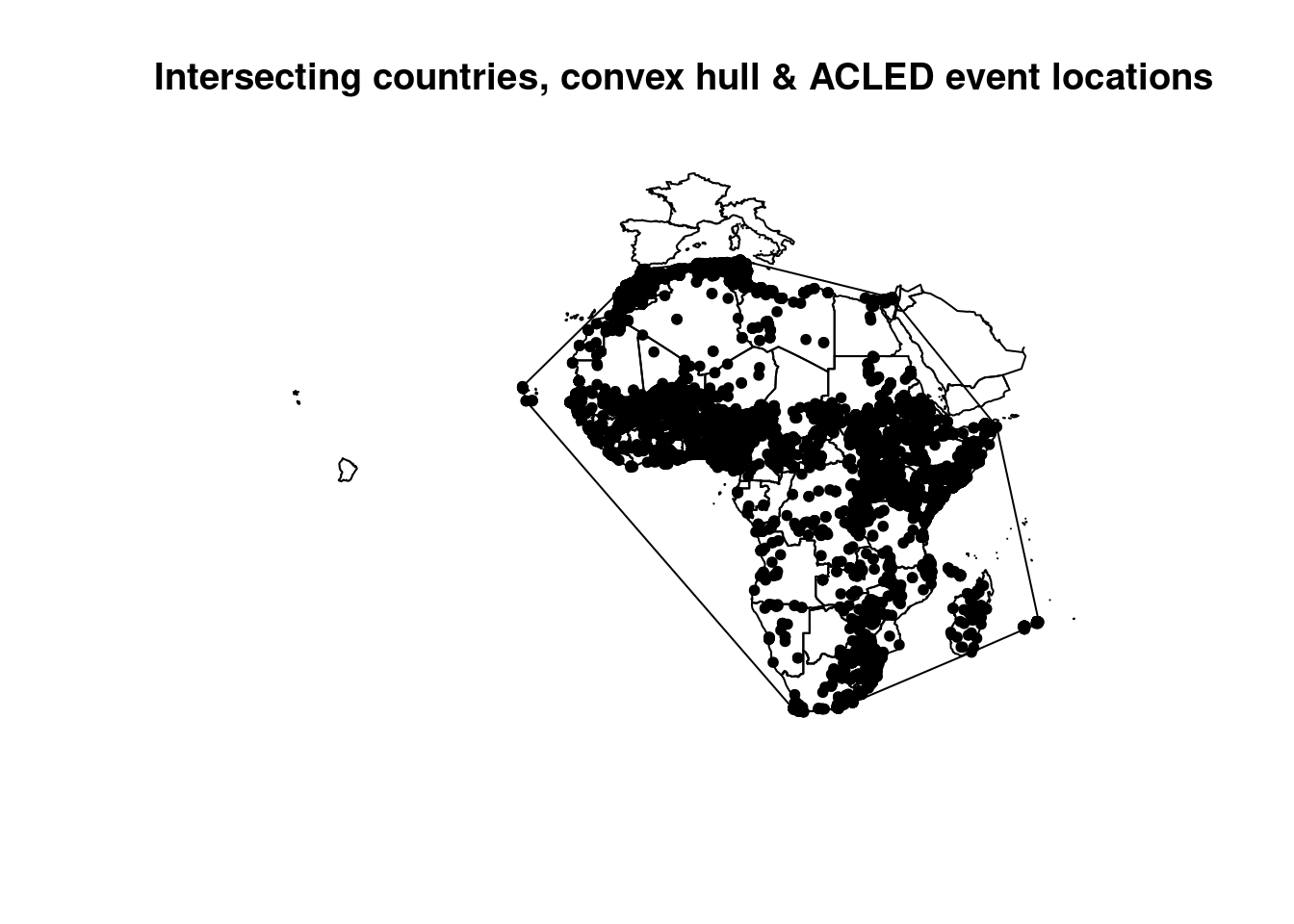
The first two lines show us how the sf predicate works. The first is a sparse spatial predicate list which, as mentioned, lists the Id’s for which features of the second dataset the predicate is TRUE. Whereas the second line creates a so called dense logical matrix. The matrix combines all features (our convex hull is a single feature) and contains information if the predicate is TRUE or FALSE. When used in a dplyr filter function, you need a dense logical matrix, a sparse predicate list wont work to filter. No need to add st_intersects(A,B)==TRUE.
4.2.5 Point in polygon and buffer
We successfully applied a spatial filter on the country dataset. Next we count the events per country boundary. The algorithm behind is called point in polygon (PIP).
## Sparse geometry binary predicate list of length 62, where the predicate
## was `intersects'
## first 10 elements:
##  1: (empty)
##  2: (empty)
##  3: (empty)
##  4: 764, 765, 766, 767, 768, 769, 770, 771, 772, 773
##  5: 2266, 2267, 2268, 2269, 2270, 2272, 2273, 2274, 2275, 2276, ...
##  6: 3138, 3139, 3140, 3141, 3142, 3143, 3144, 3145, 3146, 3147, ...
##  7: 3044, 3045, 3046, 3047, 3048, 3049, 3050, 3051, 3052, 3053, ...
##  8: 8991
##  9: 2492, 2493, 2494, 2495, 2496, 2497, 2498, 2499, 2500, 2501, ...
## 10: 2458, 2459, 2460, 2461, 2462, 2463, 2464, 2465, 2466, 2467, ...## [1] 0 0 0 10 14 76 94 1 516 34 52 3 1465 86 0
## [16] 8 81 503 38 132 901 230 0 20 85 55 50 148 137 313
## [31] 965 0 85 597 1018 17 2 0 38 101 0 205 219 0 0
## [46] 117 41 508 1 61 2 3 13 68 159 26 833 7 43 403
## [61] 3 27In the code chunk above we use the sparse predicates output of st_intersects and simply count the list of intersecting feature ids of B per feature in A
lengths() converts the sparse predicate list of intersecting ids into a count.
In the next chunk we compare our PIP result with a non-spatial aggregation based on the COUNTRY attribute in ACLED.
countries.intersects |>
  dplyr::select(shapeName, event_count) |>
  arrange(desc(event_count)) |>
  head()
## Simple feature collection with 6 features and 2 fields
## Geometry type: MULTIPOLYGON
## Dimension: XY
## Bounding box: xmin: -5.513213 ymin: -34.83324 xmax: 51.41463 ymax: 22.22488
## Geodetic CRS: WGS 84
## shapeName event_count geometry
## 1 Nigeria 1465 MULTIPOLYGON (((7.062879 13...
## 2 Democratic Republic of the Congo 1018 MULTIPOLYGON (((12.56832 -6...
## 3 Burkina Faso 965 MULTIPOLYGON (((-0.4860051 ...
## 4 Sudan 901 MULTIPOLYGON (((38.40776 18...
## 5 Somalia 833 MULTIPOLYGON (((41.85871 3....
## 6 South Africa 597 MULTIPOLYGON (((32.88588 -2...acled_africa.sf |>
ungroup() |>
group_by(COUNTRY) |>
summarise(event_count=n()) |>
arrange(desc(event_count)) |>
head()## Simple feature collection with 6 features and 2 fields
## Geometry type: MULTIPOINT
## Dimension: XY
## Bounding box: xmin: -4.971 ymin: -34.532 xmax: 51.038 ymax: 21.998
## Geodetic CRS: WGS 84
## # A tibble: 6 × 3
## COUNTRY event_count geometry
## <chr> <int> <MULTIPOINT [°]>
## 1 Nigeria 1465 ((4.509 9.883), (4.724 10.187), (4.6…
## 2 Democratic Republic of Congo 1018 ((18.271 0.047), (22.45 0.583), (19.…
## 3 Burkina Faso 963 ((-1.252 14.548), (-1.274 14.289), (…
## 4 Sudan 898 ((22.45 13.183), (22.186 13.123), (2…
## 5 Somalia 858 ((43.009 10.091), (44.067 9.56), (43…
## 6 South Africa 598 ((18.757 -32.903), (18.625 -31.776),…The first two records are identical. Some minor differences are present however. Possible sources of this can either be the selected predicate or the methodology. Intersects predicate is also true if two geometries are only touching each other. So, events that are exactly located at the border are also counted. The COUNTRY attribute is not necessary the depicting the location of an event, but the country of actors and addresses.
For the next example of a simple buffer analysis, we load a dataset based on the Kreise or districts with the weekly COVID incidence rate.
## Reading layer `kreiseWithCovidMeldeWeeklyCleaned' from data source
##   `/home/slautenbach/Documents/lehre/HD/git_areas/spatial_data_science/spatial-data-science/data/covidKreise.gpkg'
##   using driver `GPKG'
## Simple feature collection with 400 features and 145 fields
## Geometry type: MULTIPOLYGON
## Dimension:     XY
## Bounding box:  xmin: 280371.1 ymin: 5235856 xmax: 921292.4 ymax: 6101444
## Projected CRS: ETRS89 / UTM zone 32N## [1] "RS_0" "EWZ"
## [3] "GEN" "GF"
## [5] "BEZ" "ADE"
## [7] "BSG" "ARS"
## [9] "AGS" "SDV_ARS"
## [11] "ARS_0" "AGS_0"
## [13] "RS" "IdLandkreis"
## [15] "casesWeek_2020_01_02" "casesWeek_2020_01_23"
## [17] "casesWeek_2020_02_01" "casesWeek_2020_02_07"
## [19] "casesWeek_2020_02_15" "casesWeek_2020_02_20"
## [21] "casesWeek_2020_03_01" "casesWeek_2020_03_08"
## [23] "casesWeek_2020_03_15" "casesWeek_2020_03_22"
## [25] "casesWeek_2020_03_29" "casesWeek_2020_04_05"
## [27] "casesWeek_2020_04_12" "casesWeek_2020_04_19"
## [29] "casesWeek_2020_04_26" "casesWeek_2020_05_03"
## [31] "casesWeek_2020_05_10" "casesWeek_2020_05_17"
## [33] "casesWeek_2020_05_24" "casesWeek_2020_05_31"
## [35] "casesWeek_2020_06_07" "casesWeek_2020_06_14"
## [37] "casesWeek_2020_06_21" "casesWeek_2020_06_28"
## [39] "casesWeek_2020_07_05" "casesWeek_2020_07_12"
## [41] "casesWeek_2020_07_19" "casesWeek_2020_07_26"
## [43] "casesWeek_2020_08_02" "casesWeek_2020_08_09"
## [45] "casesWeek_2020_08_16" "casesWeek_2020_08_23"
## [47] "casesWeek_2020_08_30" "casesWeek_2020_09_06"
## [49] "casesWeek_2020_09_13" "casesWeek_2020_09_20"
## [51] "casesWeek_2020_09_27" "casesWeek_2020_10_04"
## [53] "casesWeek_2020_10_11" "casesWeek_2020_10_18"
## [55] "casesWeek_2020_10_25" "casesWeek_2020_11_01"
## [57] "casesWeek_2020_11_08" "casesWeek_2020_11_15"
## [59] "casesWeek_2020_11_22" "casesWeek_2020_11_29"
## [61] "casesWeek_2020_12_06" "casesWeek_2020_12_13"
## [63] "casesWeek_2020_12_20" "casesWeek_2020_12_27"
## [65] "casesWeek_2021_01_03" "casesWeek_2021_01_10"
## [67] "casesWeek_2021_01_17" "casesWeek_2021_01_24"
## [69] "casesWeek_2021_01_31" "casesWeek_2021_02_07"
## [71] "casesWeek_2021_02_14" "casesWeek_2021_02_21"
## [73] "casesWeek_2021_02_28" "casesWeek_2021_03_07"
## [75] "casesWeek_2021_03_14" "casesWeek_2021_03_21"
## [77] "casesWeek_2021_03_28" "casesWeek_2021_04_04"
## [79] "casesWeek_2021_04_11" "casesWeek_2021_04_18"
## [81] "casesWeek_2021_04_25" "casesWeek_2021_05_02"
## [83] "casesWeek_2021_05_09" "casesWeek_2021_05_16"
## [85] "casesWeek_2021_05_23" "casesWeek_2021_05_30"
## [87] "casesWeek_2021_06_06" "casesWeek_2021_06_13"
## [89] "casesWeek_2021_06_20" "casesWeek_2021_06_27"
## [91] "casesWeek_2021_07_04" "casesWeek_2021_07_11"
## [93] "casesWeek_2021_07_18" "casesWeek_2021_07_25"
## [95] "casesWeek_2021_08_01" "casesWeek_2021_08_08"
## [97] "casesWeek_2021_08_15" "casesWeek_2021_08_22"
## [99] "casesWeek_2021_08_29" "casesWeek_2021_09_05"
## [101] "casesWeek_2021_09_12" "casesWeek_2021_09_19"
## [103] "casesWeek_2021_09_26" "casesWeek_2021_10_03"
## [105] "casesWeek_2021_10_10" "casesWeek_2021_10_17"
## [107] "casesWeek_2021_10_24" "casesWeek_2021_10_31"
## [109] "casesWeek_2021_11_07" "casesWeek_2021_11_14"
## [111] "casesWeek_2021_11_21" "casesWeek_2021_11_28"
## [113] "casesWeek_2021_12_05" "casesWeek_2021_12_12"
## [115] "casesWeek_2021_12_19" "casesWeek_2021_12_26"
## [117] "casesWeek_2022_01_02" "casesWeek_2022_01_09"
## [119] "casesWeek_2022_01_16" "casesWeek_2022_01_23"
## [121] "casesWeek_2022_01_30" "casesWeek_2022_02_06"
## [123] "casesWeek_2022_02_13" "casesWeek_2022_02_20"
## [125] "casesWeek_2022_02_27" "casesWeek_2022_03_06"
## [127] "casesWeek_2022_03_13" "casesWeek_2022_03_20"
## [129] "casesWeek_2022_03_27" "casesWeek_2022_04_03"
## [131] "casesWeek_2022_04_10" "casesWeek_2022_04_17"
## [133] "casesWeek_2022_04_24" "casesWeek_2022_04_27"
## [135] "sumCasesTotal" "incidenceTotal"
## [137] "Langzeitarbeitslosenquote" "Hochqualifizierte"
## [139] "Breitbandversorgung" "Stimmenanteile.AfD"
## [141] "Studierende" "Einpendler"
## [143] "Auspendler" "Auslaenderanteil"
## [145] "Laendlichkeit" "geom"st_read is the function of sf to read in spatial file formats. It supports all common file formats. Some of them might contain layers, as the GeoPackage we open in the example. The layer is defined by the parameter layer. The equivalent for writing sf dataframes is st_write().
Explanation of attributes:
- GEN - Name of the Kreis
- EWZ - Amount of inhabitants
- casesWeek_ - 7 day amount of infected people.
- sumCasesTotal - Total cases up to the end of April
- incidenceTotal - Total incidence rate at the end of April
- Langzeitarbeitslosenquote - Long-term (> 1 year) unemployment rate
- Hochqualifizierte - Rate of high qualified workforce
- Breitbandversorgung - Broadband supply rate
- Stimmenanteile.AfD - Share of voes for the political party AFD
- Studierende - Rate of students
- Einpendler - Rate of workforce commuting into a Kreis
- Auspendler - Rate of workforce commuting outside a Kreis
- Auslaenderanteil - Rate of foreign population
- Laendlichkeit - Score of rurality / remoteness
- geom - geometric boundary of a Kreis
How many Kreise are within a 50km radius of the centroid of Berlin?
## Warning: st_centroid assumes attributes are constant over geometriesberlin_buffer50 <- berlin |>
st_transform(32632) |>
st_buffer(50000)
covidKreise |> st_transform(32632) |>
filter(st_intersects(geom, berlin_buffer50, sparse=F)) |>
dplyr::select(GEN, EWZ) |>
arrange(desc(EWZ))## Simple feature collection with 12 features and 2 fields
## Geometry type: MULTIPOLYGON
## Dimension: XY
## Bounding box: xmin: 709972.3 ymin: 5741117 xmax: 894627.9 ymax: 5913170
## Projected CRS: WGS 84 / UTM zone 32N
## First 10 features:
## GEN EWZ geom
## 1 Berlin 3669491 MULTIPOLYGON (((802565.3 58...
## 2 Potsdam-Mittelmark 216566 MULTIPOLYGON (((736431.9 58...
## 3 Oberhavel 212914 MULTIPOLYGON (((779197.5 59...
## 4 Märkisch-Oderland 195751 MULTIPOLYGON (((844617.2 58...
## 5 Barnim 185244 MULTIPOLYGON (((825694.2 58...
## 6 Potsdam 180334 MULTIPOLYGON (((772180.6 58...
## 7 Oder-Spree 178803 MULTIPOLYGON (((852096.6 58...
## 8 Dahme-Spreewald 170791 MULTIPOLYGON (((804682.2 58...
## 9 Teltow-Fläming 169997 MULTIPOLYGON (((797356.5 58...
## 10 Havelland 162996 MULTIPOLYGON (((742792.5 58...First we filter for Berlin and convert the boundary geometry into a centroid. For the buffer analysis it is necessary to work in a projected metric system to define the buffer radius in meter. Otherwise we are stuck with decimal degrees. Then we use the 50km buffer around Berlin to filter again with st_intersects.
## Coordinate Reference System:
##   User input: EPSG:32632
##   wkt:
## PROJCRS["WGS 84 / UTM zone 32N",
##     BASEGEOGCRS["WGS 84",
##         ENSEMBLE["World Geodetic System 1984 ensemble",
##             MEMBER["World Geodetic System 1984 (Transit)"],
##             MEMBER["World Geodetic System 1984 (G730)"],
##             MEMBER["World Geodetic System 1984 (G873)"],
##             MEMBER["World Geodetic System 1984 (G1150)"],
##             MEMBER["World Geodetic System 1984 (G1674)"],
##             MEMBER["World Geodetic System 1984 (G1762)"],
##             MEMBER["World Geodetic System 1984 (G2139)"],
##             ELLIPSOID["WGS 84",6378137,298.257223563,
##                 LENGTHUNIT["metre",1]],
##             ENSEMBLEACCURACY[2.0]],
##         PRIMEM["Greenwich",0,
##             ANGLEUNIT["degree",0.0174532925199433]],
##         ID["EPSG",4326]],
##     CONVERSION["UTM zone 32N",
##         METHOD["Transverse Mercator",
##             ID["EPSG",9807]],
##         PARAMETER["Latitude of natural origin",0,
##             ANGLEUNIT["degree",0.0174532925199433],
##             ID["EPSG",8801]],
##         PARAMETER["Longitude of natural origin",9,
##             ANGLEUNIT["degree",0.0174532925199433],
##             ID["EPSG",8802]],
##         PARAMETER["Scale factor at natural origin",0.9996,
##             SCALEUNIT["unity",1],
##             ID["EPSG",8805]],
##         PARAMETER["False easting",500000,
##             LENGTHUNIT["metre",1],
##             ID["EPSG",8806]],
##         PARAMETER["False northing",0,
##             LENGTHUNIT["metre",1],
##             ID["EPSG",8807]]],
##     CS[Cartesian,2],
##         AXIS["(E)",east,
##             ORDER[1],
##             LENGTHUNIT["metre",1]],
##         AXIS["(N)",north,
##             ORDER[2],
##             LENGTHUNIT["metre",1]],
##     USAGE[
##         SCOPE["Navigation and medium accuracy spatial referencing."],
##         AREA["Between 6°E and 12°E, northern hemisphere between equator and 84°N, onshore and offshore. Algeria. Austria. Cameroon. Denmark. Equatorial Guinea. France. Gabon. Germany. Italy. Libya. Liechtenstein. Monaco. Netherlands. Niger. Nigeria. Norway. Sao Tome and Principe. Svalbard. Sweden. Switzerland. Tunisia. Vatican City State."],
##         BBOX[0,6,84,12]],
##     ID["EPSG",32632]]
EPSG:32632 is a projection of the UTM system. It is Zone 32N and covers Germany.
4.2.6 Spatial aggregation
Another common GIS operation is Union. Sometimes it is also referred to as dissolve, as it literally dissolves boundaries between adjacent geometries. This dissolving can be controlled by one or multiple attributes. Features that share the same value in the defined attribute will be unionend / dissolved into one. We use the COVID Kreise dataset to create Bundesländer geometries and aggregate the case numbers for the last week in April.
## Geometry set for 1 feature
## Geometry type: MULTIPOLYGON
## Dimension:     XY
## Bounding box:  xmin: 280371.1 ymin: 5235856 xmax: 921292.4 ymax: 6101444
## Projected CRS: ETRS89 / UTM zone 32N
## MULTIPOLYGON (((420089.7 5433027, 420065.3 5432...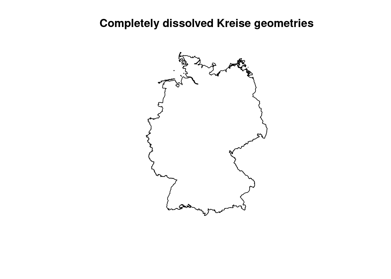
covidBundesland <- covidKreise |>
  group_by(substr(RS, 1,2)) |>
  summarise(
    EWZ=sum(EWZ),
    casesWeek_2022_04_27 = sum(casesWeek_2022_04_27),
    geom=st_union(geom)) |>
  arrange(desc(EWZ))

covidBundesland
## Simple feature collection with 16 features and 3 fields
## Geometry type: GEOMETRY
## Dimension: XY
## Bounding box: xmin: 280371.1 ymin: 5235856 xmax: 921292.4 ymax: 6101444
## Projected CRS: ETRS89 / UTM zone 32N
## # A tibble: 16 × 4
## `substr(RS, 1, 2)` EWZ casesWeek_2022_04_27 geom
## <chr> <dbl> <int> <GEOMETRY [m]>
## 1 05 17947221 62848 MULTIPOLYGON (((300866.8 56…
## 2 09 13124737 53275 POLYGON ((609367.6 5267771,…
## 3 08 11100394 42795 MULTIPOLYGON (((462908.5 52…
## 4 03 7993608 44880 MULTIPOLYGON (((427439.2 57…
## 5 06 6288080 31157 MULTIPOLYGON (((477311.8 54…
## 6 07 4093903 18080 POLYGON ((420282.7 5433036,…
## 7 14 4071971 12702 POLYGON ((754018.8 5589577,…
## 8 11 3669491 12210 MULTIPOLYGON (((802565.3 58…
## 9 01 2903773 17114 MULTIPOLYGON (((480100.3 59…
## 10 12 2521893 9049 MULTIPOLYGON (((785798.1 57…
## 11 15 2194782 7423 MULTIPOLYGON (((670436.8 56…
## 12 16 2133378 5699 POLYGON ((638299.7 5583419,…
## 13 02 1847253 6895 MULTIPOLYGON (((578219 5954…
## 14 13 1608138 5043 MULTIPOLYGON (((721682.5 59…
## 15 10 986887 4402 POLYGON ((361400.9 5446494,…
## 16 04 681202 2558 MULTIPOLYGON (((467379.6 58…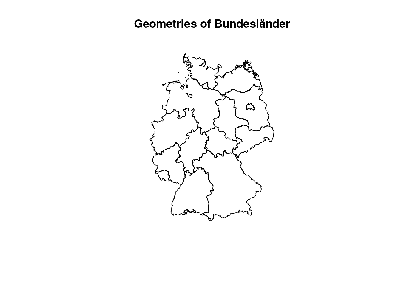
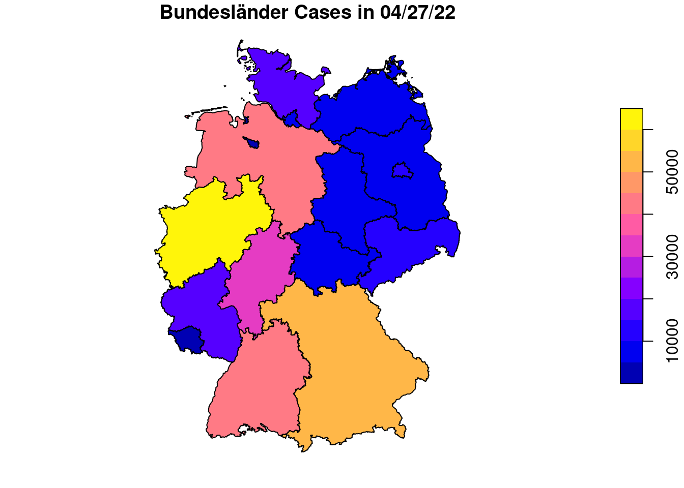
Applied on the COVID Kreise Dataset all geometries are dissolved into a single polygon which represents Germany then. We did the same with the ACLED event data, before creating a convex hull around it. By the group_by function we define groups which the features are assigned to will then get unionend. We use the RS attribute which is a combined identification number for each Kreis. The first two digits bears information on the Bundesland. Therefore we subset the digit and use it then for the group_by function. Attributes on population and cases are just summed up, on the geometry the union function is applied.
4.3 Raster data
4.3.1 Read raster data, geometric operations
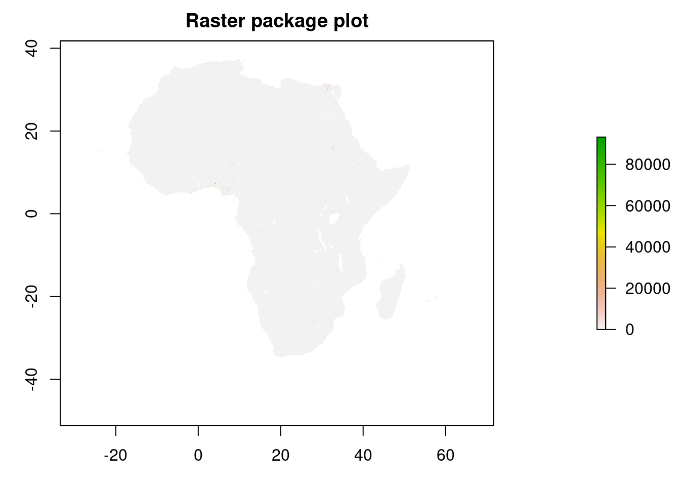
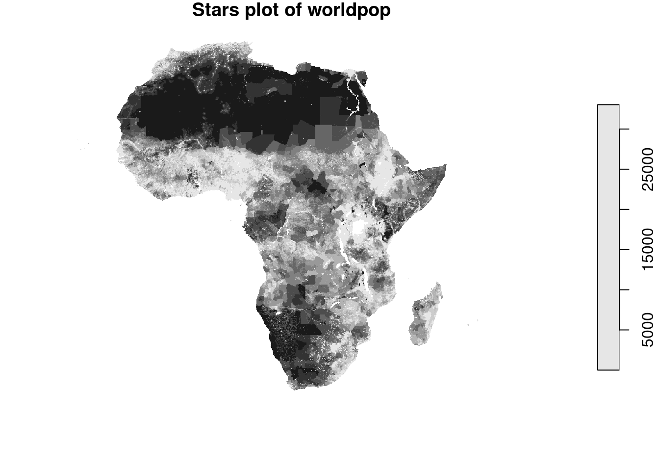
Next we take a look at raster data in R. First we load in a geotiff file from WorldPop that covers population counts for Africa at 1km resolution.
## terra 1.8.15## Loading required package: sp##
## Attaching package: 'raster'## The following object is masked from 'package:dplyr':
##
## select## Loading required package: abindwpop <- rast("data/AFR_PPP_2020_adj_v2.tif")
wpop_ras <- as(wpop, "Raster")
wpop_stars <- aggregate(wpop, fact = 10, fun = mean) %>% st_as_stars() # downsamply by a factor of 10 to speed up plotting##
|---------|---------|---------|---------|
=========================================
## class      : RasterLayer
## dimensions : 11161, 12575, 140349575  (nrow, ncol, ncell)
## resolution : 0.008333333, 0.008333333  (x, y)
## extent     : -33.32542, 71.46625, -51.21708, 41.79125  (xmin, xmax, ymin, ymax)
## crs        : +proj=longlat +datum=WGS84 +no_defs
## source     : AFR_PPP_2020_adj_v2.tif
## names : AFR_PPP_2020_adj_v2## stars object with 2 dimensions and 1 attribute
## attribute(s), summary of first 1e+05 cells:
## Min. 1st Qu. Median Mean 3rd Qu. Max. NA's
## AFR_PPP_2020_adj_v2 2.039894 14.8136 35.66279 134.4454 116.71 7388.898 97307
## dimension(s):
## from to offset delta refsys x/y
## x 1 1258 -33.33 0.08333 WGS 84 [x]
## y 1 1117 41.79 -0.08333 WGS 84 [y]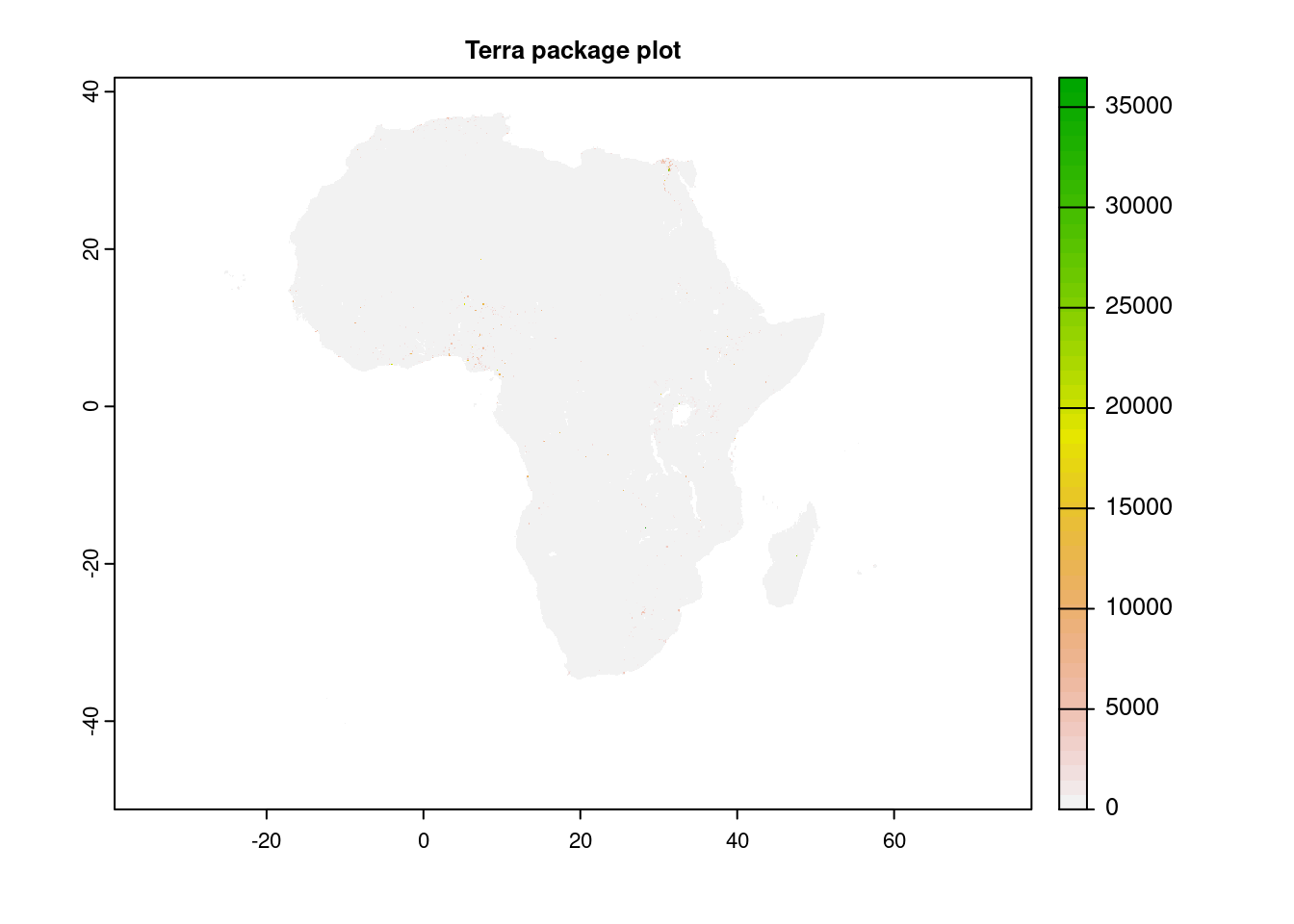
plot(wpop, breaks=c(0,1,5,10,50,100,500,1000), main="Classified population values") # cell values as fixed classes, not continuous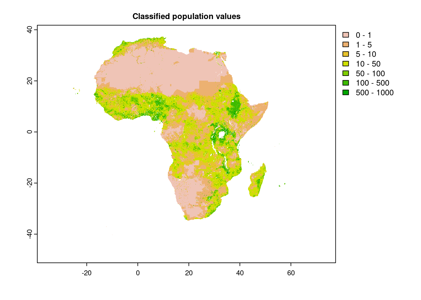
When loading the raster package, R tells us that the function select is masked from the dplyr package.
This means that the raster package also defines aa function with the name select. When we now apply select in our workflow, the raster select is used. If we want to use the dplyr one we need to write this explicitly dplyr::select. Another way is to detach both packages and first call the raster and then the dplyr package. However, if raster has been imported by another package (as in our case, it cannot be unloaded if the calling package is not detached as well.
In the chunk above you see how raster files in the different libraries are represented in R. To read/write raster data use the following commands:
x <- terra:rast("path/to/rasterfile.tif")
x <- raster:raster("path/to/rasterfile.tif")
x <- stars::read_stars("path/to/rasterfile.tif", proxy=F)

stars::write_stars(x, "path/to/rasterfile.tif", proxy=F)
raster:writeRaster(x, "path/to/rasterfile.tif")
terra:writeRaster(x, "path/to/rasterfile.tif")
If you read in a multiband raster each band is represented as a layer of the raster object and can be referenced to via the $ like: x$layer
The next code chunk shows how to cut rasters to a desired area, defined by e.g. an sf object.
countries_of_interest <- c("Namibia", "South Africa", "Botswana", "Lesotho", "Eswatini")

# get a subset of countries
countries.intersects.subset <- countries.intersects |>
  filter(shapeName %in% countries_of_interest)

# crop
wpop |> crop(countries.intersects.subset) |>
  plot()
plot(countries.intersects.subset$geometry, add=T)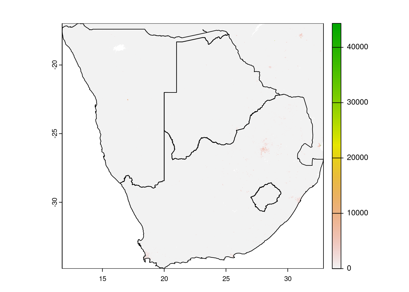
# crop + mask
wpop |> crop(countries.intersects.subset) |>
  mask(vect(countries.intersects.subset)) |>
  plot()
plot(countries.intersects.subset$geometry, add=T)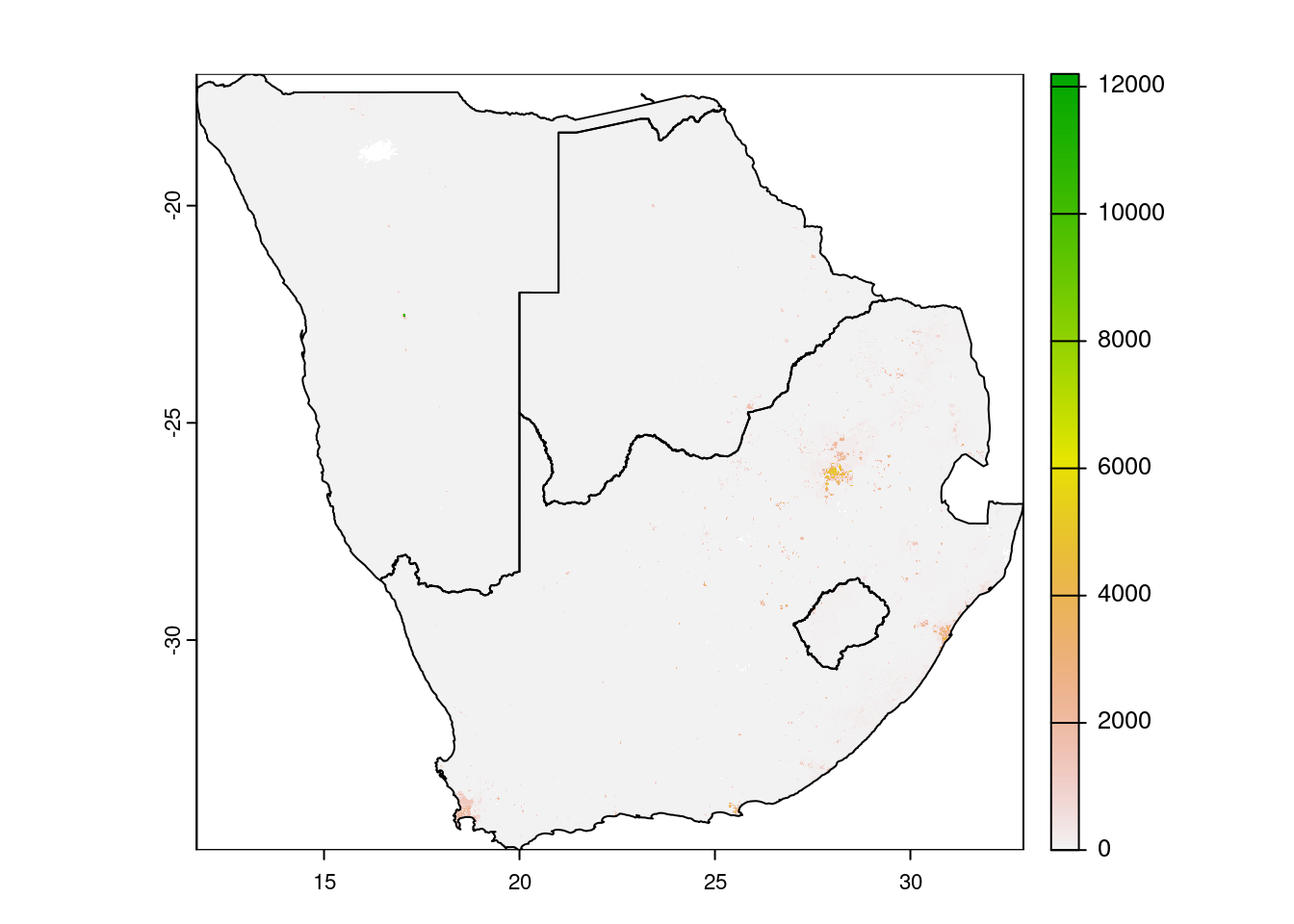
First we filter for a selection of countries by name. This selection of country geometries is then used with the crop() function. Crop will use the extent of the vector to cut the raster. Mask does the same but also sets cells that are not covered by the masking vector to either NA or a defined value. The crop function accepts sf dataframes, the mask function not. You need to convert it to a SpatVector class, from the terra package.
4.3.2 Zonal statistics
All of the raster packages have capabilities to perform zonal statistics.
We prefer the exactextractr package because of its great performance even with larger datasets and extended parameter options. You can set how to handle cells that are not completely in only one zone of the vector layer. For example you configure to distribute the cell value by area or by a weight based on another raster band. For more infos on the underlying exactextract software, consult the github repository.
library(exactextractr)
countries.intersects.subset$wpop <- exact_extract(wpop, countries.intersects.subset, fun="sum")
##
|
| | 0%
|
|================== | 25%
|
|=================================== | 50%
|
|==================================================== | 75%
|
|======================================================================| 100%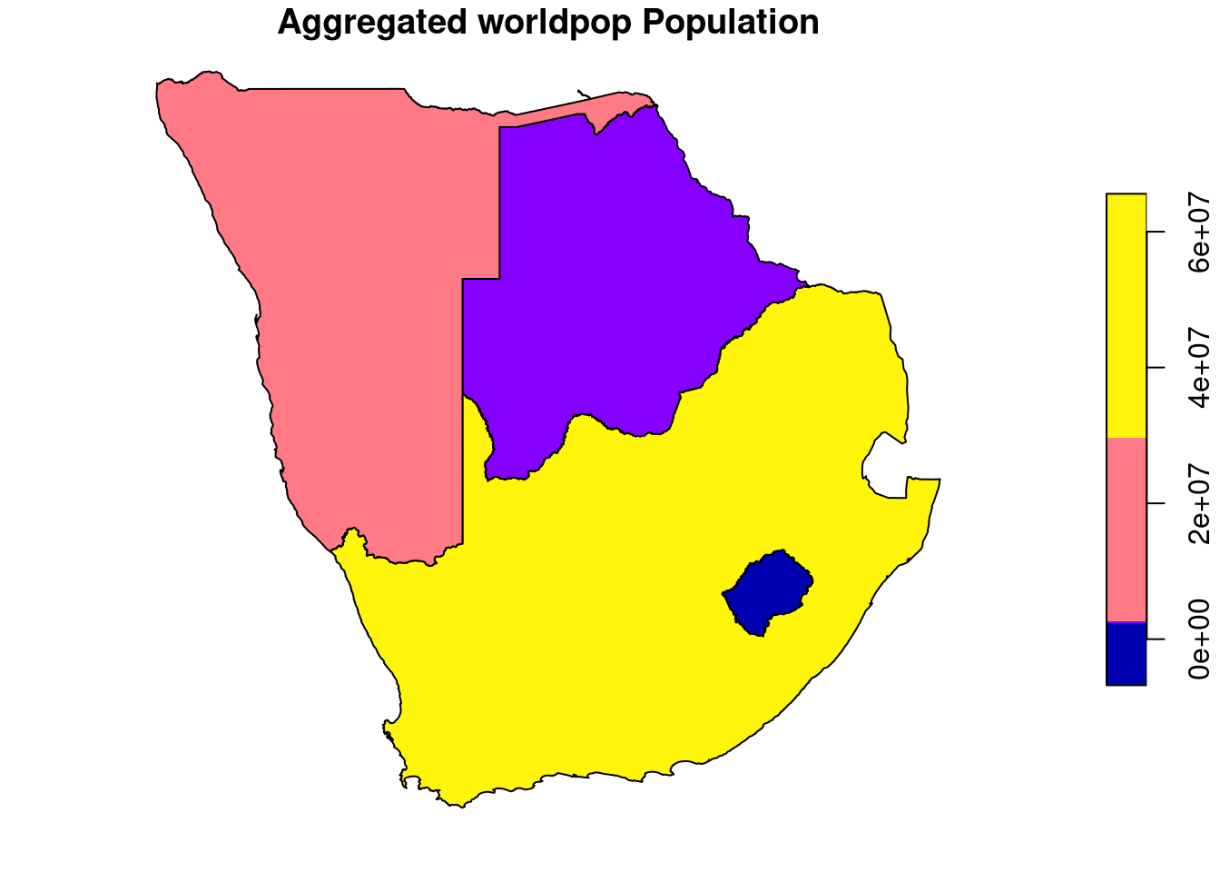
Exact extract can work with terra raster objects out of the box, no need for conversion back to a raster package object.
A new column wpop is added and filled with the result of the operator applied on all cells within a feature / zone. Sum is only one of many operators that can be looked up via the documentation of exactextract ?exactextratr::exact_extract().
4.4 Mapmaking
Up to now we did some more or less pretty but helpful plots mainly to explore our datasets or to verify outputs of applied functions. The R base plot() function and its implementation in sf and the raster packages is already powerful to visualize spatial data and with some effort on setting additional parameters, a decent map can be created. However there are other more advanced packages to create more sophisticated maps. And of course one major advantage of using R for mapmaking is its scalability via loops, user-defined functions and parameterization.
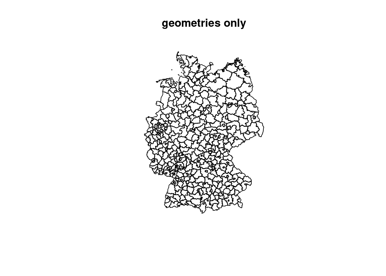
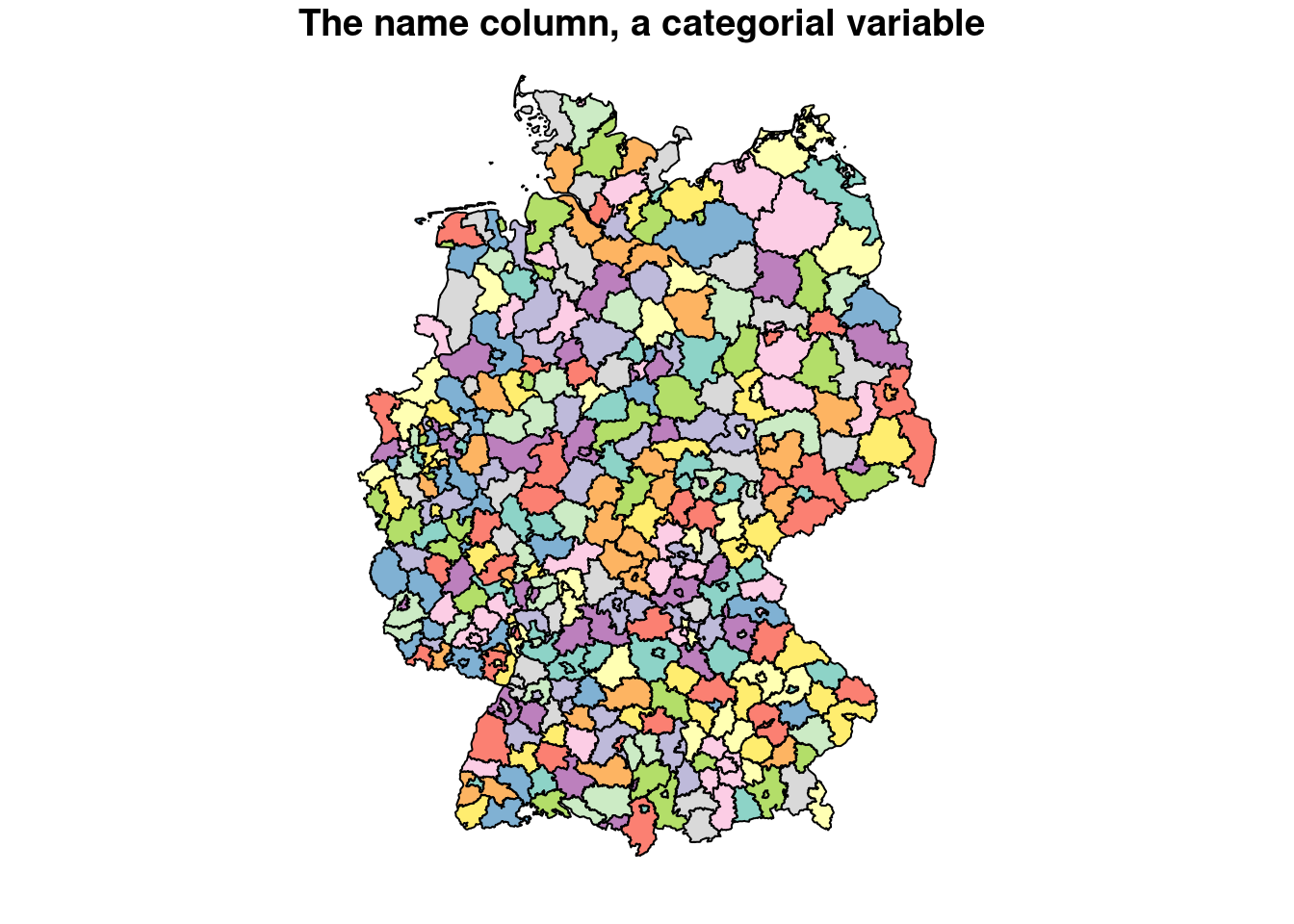
plot(covidKreise["casesWeek_2022_04_27"], main="Cases in 04/27/22, numeric variable") # numerical variable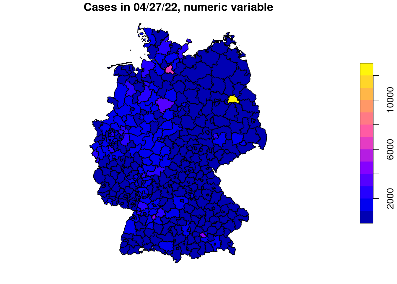
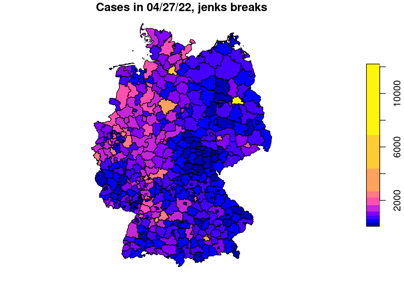
plot(covidKreise["casesWeek_2022_04_27"], main="Cases in 04/27/22, equal interval", breaks="equal" )
4.4.1 Interactive maps
During the exploration or experimental phase of a R project it is good practice to youse map visualizations to explore, investigate and verify spatial data. Beside the standard plot() function with simple styling, interactive maps can support a more detailed investigation of the data, especially if it covers a large extent.
Libraries to use for quick interactive maps are mapview and tmap.
Note: currently disabled interactive mapping due to issues then compiling the book
library(mapview)
mapview(acled_africa.sf, zcol="EVENT_TYPE")

tmap_mode("view")
tm_shape(acled_africa.sf) +
  tm_dots("EVENT_TYPE")
Mapview out of the box pop ups all attribute information when clicking on a features location. To use Tmap for interactive maps, one has to activate the view mode by executing the command: tmap_mod("view"). Tmap is a powerful library to create thematic maps. Not only interactive, but static ready to be exported as rasterized image or vector file ready to be fine tuned in a vector graphics software like Inkscape or Ilustrator.
4.4.2 Static maps with tmap
## ℹ tmap mode set to "plot".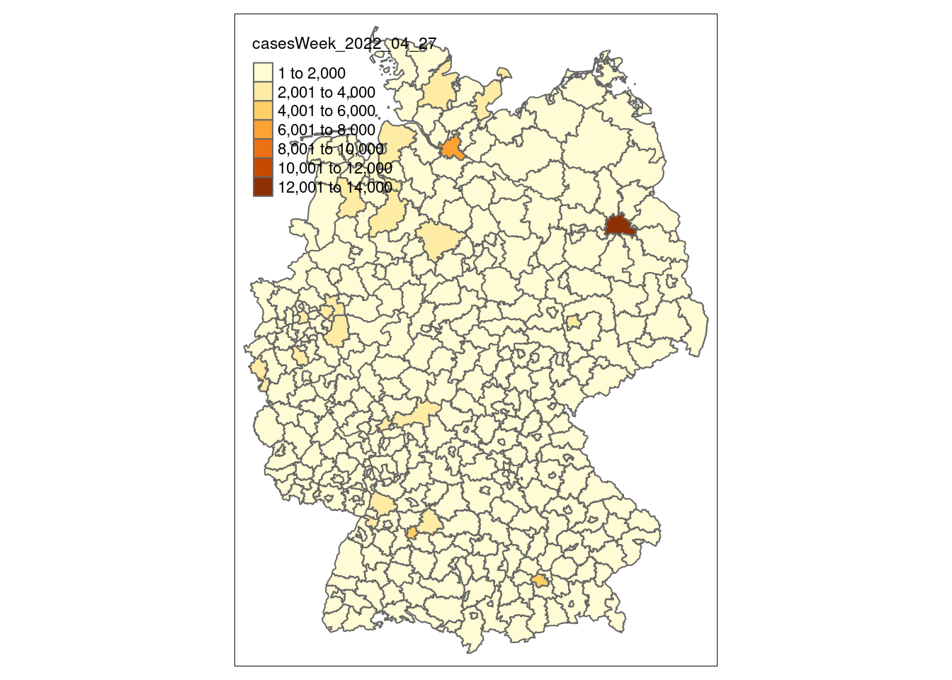
Tmap follows a different syntax than base R and piping, comparable to ggplot. Every tmap plot starts with the tm_shape() command which defines the spatial dataset to be used as first layer that is dran in the map. Every subsequent added tm_shape will be drawn as separate layer on top. Depending on the geometry tmap offers different tmap-elements for visualization. Polygons for example can be drawn with tm_polygon where you can define a fill and border color. You can also just use the tmap-element tm_fill or tm_borders. For line geometries tm_lines. For points tm_symbols, tm_dots, tm_dots or tm_markers among others. Raster layer are visualized via tm_raster, multiband raster can be assigned red, green, blue per band via tm_rgb. Other map elements can be added via tm_scale_bar, tm_compass. The legend can be configured via the corresponding tmap layer elements and with tm_layout. There you an also configure general map settings.
With the command tmaptools::palette_explorer() a graphical user interface can be started to explore different color ramps. When using a colorramp, putting a - in front will invert the color order.
tm_shape(covidKreise) + # spatial dataframe
  tm_polygons(  # type of visualization. for vectors: polygons, lines/borders, dots/symbols
    "casesWeek_2022_04_27", # attribute field
    breaks = c(0, 100, 200, 500, 1000, 2000, 4000, 6000, 13000), # class breaks
    legend.hist = TRUE, # show a histogram
    legend.reverse = T, # reverse the legend
    palette = "-plasma", # use plasma color ramp
    title = "Cases 27/04/2022" # legend title
  ) +
  tm_layout(
    legend.show = T,
    legend.outside = TRUE,
    bg.color = "darkgrey",
    outer.bg.color = "lightgrey",
    attr.outside = TRUE,
    legend.hist.width = .5,
    legend.hist.height = .5,
    legend.outside.position = "left"
  ) +
  tm_shape(covidBundesland) +
  tm_borders(lwd = 1, col="black") +
  tm_scale_bar()
## ## ── tmap v3 code detected ───────────────────────────────────────────────────────## [v3->v4] `tm_tm_polygons()`: migrate the argument(s) related to the scale of
## the visual variable `fill` namely 'breaks', 'palette' (rename to 'values') to
## fill.scale = tm_scale(<HERE>).
## [v3->v4] `tm_polygons()`: migrate the argument(s) related to the legend of the
## visual variable `fill` namely 'title', 'legend.reverse' (rename to 'reverse')
## to 'fill.legend = tm_legend(<HERE>)'
## [v3->v4] `tm_polygons()`: use `fill.chart = tm_chart_histogram()` instead of
## `legend.hist = TRUE`.
## ! `tm_scale_bar()` is deprecated. Please use `tm_scalebar()` instead.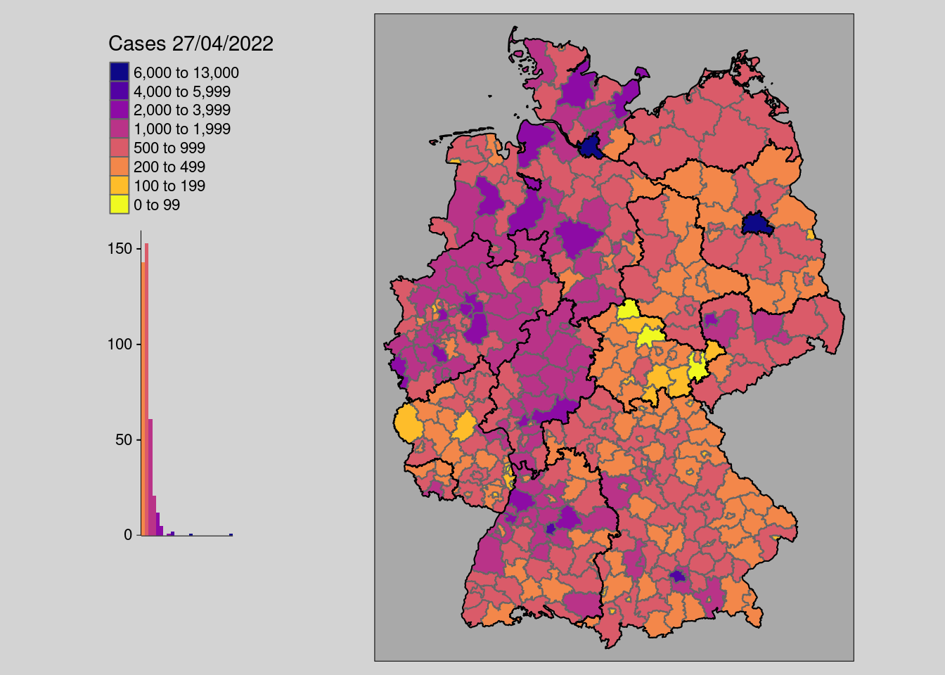
With numeric variables, it is important to create thresholds that help the reader to recognize individual features and thus patterns. You can either set them directly with the breaks= parameter like in the example above. But you can also use other parameters like n= to define the number of desired classes and style to apply an automated interval algorithm. The available algorithm in tmap come from the classint package. With the package you can also assess the interval results on a numeric input with the function: classInt::classIntervals(n = , style=).
4.5 Alternative respresentations
# filter the 10 largest kreise by area and population
covidKreise$area <- st_area(covidKreise$geom)
biggest_kreise <- covidKreise |> arrange(desc(area)) |> head(10)
most_populated_kreise <- covidKreise |> arrange(desc(EWZ))|> head(10)

t.1 <- tm_shape(covidKreise) +
  tm_borders() +
  tm_shape(biggest_kreise) +
  tm_polygons(
    "casesWeek_2022_04_27", # attribute field
    breaks = c(0, 100, 200, 500, 1000, 2000, 4000, 6000, 13000), # class breaks
    legend.hist = F,
    legend.reverse = T,
    palette = "-plasma",
  ) +
  tm_layout(
    main.title="Largest by area",
    legend.show = F,
    legend.outside = TRUE,
    bg.color = "darkgrey",
    outer.bg.color = "lightgrey",
    attr.outside = TRUE,
    legend.hist.width = .5,
    legend.hist.height = .5,
    legend.outside.position = "left"
  ) +
  tm_scale_bar()
## ## ── tmap v3 code detected ───────────────────────────────────────────────────────## [v3->v4] `tm_tm_polygons()`: migrate the argument(s) related to the scale of
## the visual variable `fill` namely 'breaks', 'palette' (rename to 'values') to
## fill.scale = tm_scale(<HERE>).
## [v3->v4] `tm_polygons()`: migrate the argument(s) related to the legend of the
## visual variable `fill` namely 'legend.reverse' (rename to 'reverse') to
## 'fill.legend = tm_legend(<HERE>)'
## [v3->v4] `tm_layout()`: use `tm_title()` instead of `tm_layout(main.title = )`
## ! `tm_scale_bar()` is deprecated. Please use `tm_scalebar()` instead.t.2 <- tm_shape(covidKreise) +
tm_borders() +
tm_shape(most_populated_kreise) +
tm_polygons(
"casesWeek_2022_04_27", # attribute field
breaks = c(0, 100, 200, 500, 1000, 2000, 4000, 6000, 13000), # class breaks
legend.hist = F,
legend.reverse = T,
palette = "-plasma",
) +
tm_layout(
main.title="Largest by pop.",
legend.show = F,
legend.outside = TRUE,
bg.color = "darkgrey",
outer.bg.color = "lightgrey",
attr.outside = TRUE,
legend.hist.width = .5,
legend.hist.height = .5,
legend.outside.position = "left"
) +
tm_scale_bar()## [v3->v4] `tm_polygons()`: migrate the argument(s) related to the legend of the
## visual variable `fill` namely 'legend.reverse' (rename to 'reverse') to
## 'fill.legend = tm_legend(<HERE>)'
## [v3->v4] `tm_layout()`: use `tm_title()` instead of `tm_layout(main.title = )`
## ! `tm_scale_bar()` is deprecated. Please use `tm_scalebar()` instead.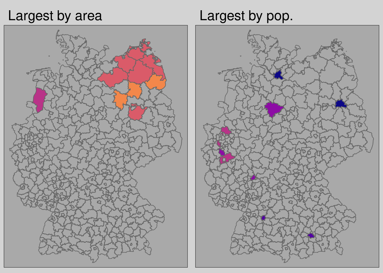
With tmap_arrange() multiple tmap objects can be used to create facet or inset maps.
- There is no direct correlation between county area and county population
- This can be problematic if for instance a couple of large areal units are affected by high incidence rates, but small populous are not
- Its the same the other way around
| Area % | Pop % | |
|---|---|---|
| Largest Units by area | 9.6 | 2.4 |
| Largest Units by pop | 2 | 15 |
4.5.1 Cartograms
With the cartograms package we can transform our areal units by the population attribute. This way we include the absolute amount of population per unit to normalize the cartogram.
- The point distribution map randomly distributes a point for every 10,000th inhabitant
- The area distorted cartogram (Dougenik et al. 1985) expands/shrinks polygons via a rubber sheet distortion algorithm
- The dorling cartogram (Dorling 1996) builds non-overlapping circles where the size represents attribute for normalization.
library(cartogram)

# point distribution map
covidKreise_pts10k <- covidKreise |>
  rowwise() |>
  mutate( # randomly distributed points inside district
    geometry=st_union(st_sample(geom, size = EWZ / 10000))
    )
# set the new geometry as the geometry to be used
st_geometry(covidKreise_pts10k) <- covidKreise_pts10k$geometry

# area distorted
covidKreise_cart <- covidKreise |>
  cartogram_cont("EWZ", itermax=10)

# dorling
covidKreise_dorling <- covidKreise |>
  cartogram_dorling("EWZ")
We store the results of the cartogram functions into separate objects as the geometry will be altered. The next chunk visualizes the cartograms with tmap.
# point distribution
tm_shape(covidKreise) +
  tm_fill(col = "grey70", lwd = .5) +
  tm_shape(covidKreise_pts10k) +
  tm_dots(
    col="casesWeek_2022_04_27", # attribute field
    breaks = c(0, 100, 200, 500, 1000, 2000, 4000, 6000, 13000),
    size = 0.01,
    shape = 20,
    palette = "-plasma",
    title = "Cases 27/04/2022" ,
    legend.col.reverse = TRUE
  ) +
  tm_shape(covidKreise) +
  tm_borders(lwd = .5) +
  tm_layout(
    main.title = "Point distribution map",
    legend.show = T,
    legend.outside = TRUE,
    bg.color = "grey95",
    outer.bg.color = "lightgrey",
    attr.outside = TRUE,
    legend.hist.width = .5,
    legend.hist.height = .5,
    legend.outside.position = "left"
  )
## ## ── tmap v3 code detected ───────────────────────────────────────────────────────## [v3->v4] `tm_tm_dots()`: migrate the argument(s) related to the scale of the
## visual variable `fill` namely 'breaks', 'palette' (rename to 'values') to
## fill.scale = tm_scale(<HERE>).
## [v3->v4] `tm_dots()`: use 'fill' for the fill color of polygons/symbols
## (instead of 'col'), and 'col' for the outlines (instead of 'border.col').
## [tm_dots()] Argument `title` unknown.
## [v3->v4] `tm_layout()`: use `tm_title()` instead of `tm_layout(main.title = )`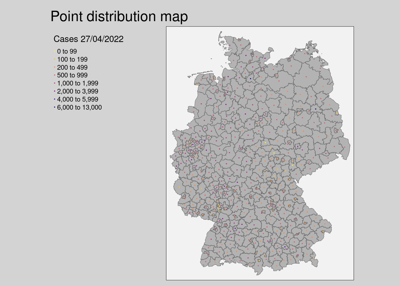
# carto
tm_shape(covidKreise_cart) +
  tm_polygons(
    "casesWeek_2022_04_27", # attribute field
    breaks = c(0, 100, 200, 500, 1000, 2000, 4000, 6000, 13000),
    legend.hist = TRUE,
    legend.reverse = T,
    palette = "-plasma",
    title = "Cases 27/04/2022"
  ) +
  tm_layout(
    main.title = "Area distorted cartogram, area by population",

    legend.show = T,
    legend.outside = TRUE,
    bg.color = "grey95",
    outer.bg.color = "lightgrey",
    attr.outside = TRUE,
    legend.hist.width = .5,
    legend.hist.height = .5,
    legend.outside.position = "left"
  )
##
## ── tmap v3 code detected ───────────────────────────────────────────────────────
## [v3->v4] `tm_tm_polygons()`: migrate the argument(s) related to the scale of
## the visual variable `fill` namely 'breaks', 'palette' (rename to 'values') to
## fill.scale = tm_scale(<HERE>).[v3->v4] `tm_polygons()`: migrate the argument(s) related to the legend of the
## visual variable `fill` namely 'title', 'legend.reverse' (rename to 'reverse')
## to 'fill.legend = tm_legend(<HERE>)'[v3->v4] `tm_layout()`: use `tm_title()` instead of `tm_layout(main.title = )`[plot mode] fit legend/component: Some legend items or map compoments do not
## fit well, and are therefore rescaled.
## ℹ Set the tmap option `component.autoscale = FALSE` to disable rescaling.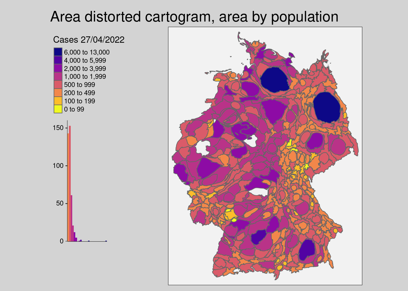
# dorling
tm_shape(covidKreise_dorling) +
  tm_polygons(
    "casesWeek_2022_04_27", # attribute field
    breaks = c(0, 100, 200, 500, 1000, 2000, 4000, 6000, 13000),
    legend.hist = TRUE,
    legend.reverse = T,
    palette = "-plasma",
    title = "Cases 27/04/2022"
  ) +
  tm_layout(
    main.title = "Dorling cartogram, area by population",
    legend.show = T,
    legend.outside = TRUE,
    bg.color = "grey95",
    outer.bg.color = "lightgrey",
    attr.outside = TRUE,
    legend.hist.width = .5,
    legend.hist.height = .5,
    legend.outside.position = "left"
  )
##
## ── tmap v3 code detected ───────────────────────────────────────────────────────
## [v3->v4] `tm_tm_polygons()`: migrate the argument(s) related to the scale of
## the visual variable `fill` namely 'breaks', 'palette' (rename to 'values') to
## fill.scale = tm_scale(<HERE>).[v3->v4] `tm_polygons()`: migrate the argument(s) related to the legend of the
## visual variable `fill` namely 'title', 'legend.reverse' (rename to 'reverse')
## to 'fill.legend = tm_legend(<HERE>)'[v3->v4] `tm_layout()`: use `tm_title()` instead of `tm_layout(main.title = )`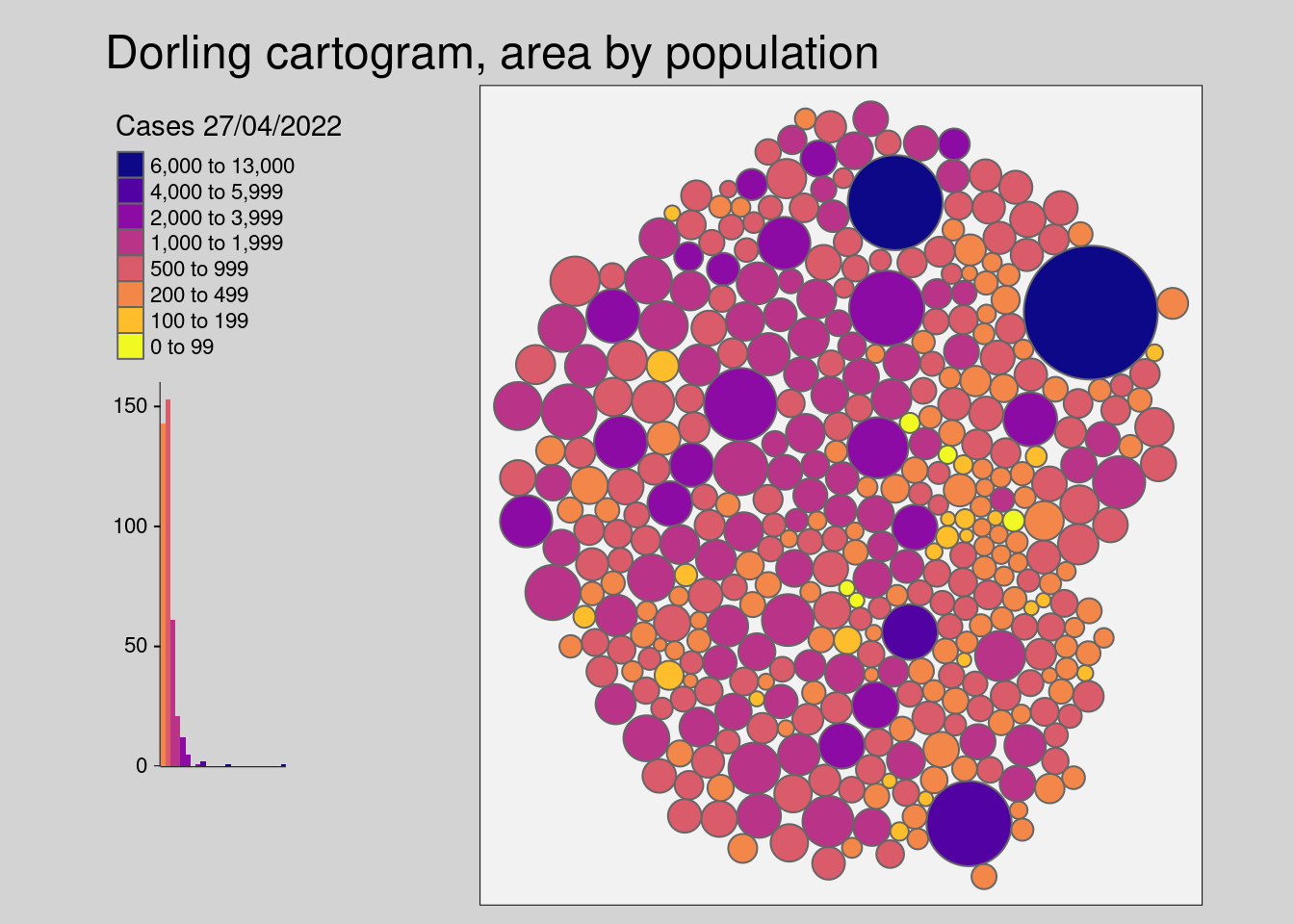
4.5.2 Animations
R provides other packages that can be used to create gifs and videos. The basic principle is to create a sequence of images, in our case maps. With R and ffmpeg we are able to produce simple animations. Here is the example of the weekly incidence rate and it’s change from the previous week.
frame_column <- names(covidKreise)[15:134] # define all columns that will be used for rendering, in sequential order

frame_title <- paste0("Incidence ",substr(names(covidKreise)[15:134],16,17), "/",substr(names(covidKreise)[15:134],19,20) , "/",substr(names(covidKreise)[15:134],11,14)) # define the titles for each frame


map <- tm_shape(covidKreise, projection = 32632) +
  tm_fill(col = frame_column,
          breaks = c(0, 100, 200, 500, 1000, 2000, 4000, 6000, 13000), # class breaks
          legend.hist = TRUE, # show a histogram
          legend.reverse = T, # reverse the legend
          palette = "-plasma", # use plasma color ramp
          title = frame_title # legend title) +
  ) +
  tm_layout(
    legend.show = T,
    legend.outside = TRUE,
    bg.color = "darkgrey",
    outer.bg.color = "lightgrey",
    attr.outside = TRUE,
    legend.hist.width = .5,
    legend.hist.height = .5,
    legend.outside.position = "left"
  )  +
  tm_facets(nrow=1,ncol=1)

tmap_animation(map, delay=20, outer.margins = 0)
## Creating frames## =## =## =## =## =## =## =## =## =## =## =## =## =## =## =## =## =## =## =## =## =## =## =## =## =## =## =## =## =## =## =## =## =## =## =## =## =## =## =## =## =## =## =## =## =## =## =## =## =## =## =## =## =## =## =## =## =## =## =## =## =## =## =## =## =## =## =## =## =## =## =## =## =## =## =## =## =## =## =## =##
## Creating animationThe chunk above is quite close to the earlier one on creating a single static map with tmap. However, instead of passing a single character value referencing the column to symbolize the map features we use a list of all columns. The order of the column names defines the order of the frames appearing sequentially in the animation. Besides the column reference, one also needs to add the tm_facets() function and use the saved tmap object in a call of the function tmap_animation. The parameter delay defines the milliseconds, a frame is visible.
This is a animation video done via printing 134 maps and combining them as frames to a single video using ffmpeg.

The table below lists selected covid related events in Germany by date.
##
## Attaching package: 'kableExtra'
## The following object is masked from 'package:dplyr':
##
## group_rowstable_event <- read.csv(header=T,text=('
"Date", "Event"
"22.02.2020","Karneval (Rheinland)"
"27.02.2020","Heinsberg Hotspot"
"09.03.2020","Ischgl Hotspot"
"18.03.2020","TV Speech Chancelor Angela Merkel"
"22.03.2020","Begin Lockdown 1"
"02.04.2020","Peak wave 1"
"12.04.2020","Easter 2020"
"15.06.2020","Tönnies Skandal"
"28.10.2020","Begin lockdown 2"
"28.10.2020","Reinforcement measures lockdown 2"
"22.12.2020","Peak wave 2"
"25.12.2020","Christmas 2020"
"04.04.2021","Easter 2021"
"23.04.2021","Begin Lockdown 3 (Bundesnotbremse)"
"25.04.2021","Peak wave 3"'))
table_event |>
kbl() |>
kable_paper("hover", full_width = T, bootstrap_options="striped")| Date | Event |
|---|---|
| 22.02.2020 | Karneval (Rheinland) |
| 27.02.2020 | Heinsberg Hotspot |
| 09.03.2020 | Ischgl Hotspot |
| 18.03.2020 | TV Speech Chancelor Angela Merkel |
| 22.03.2020 | Begin Lockdown 1 |
| 02.04.2020 | Peak wave 1 |
| 12.04.2020 | Easter 2020 |
| 15.06.2020 | Tönnies Skandal |
| 28.10.2020 | Begin lockdown 2 |
| 28.10.2020 | Reinforcement measures lockdown 2 |
| 22.12.2020 | Peak wave 2 |
| 25.12.2020 | Christmas 2020 |
| 04.04.2021 | Easter 2021 |
| 23.04.2021 | Begin Lockdown 3 (Bundesnotbremse) |
| 25.04.2021 | Peak wave 3 |
4.5.3 Bivariate maps
In a later session we will assess what socio-economic factors may be linked to incidence rates. A simple first approach to visually compare the relation of two variables is a bivariate map. The two variables are classified into three quantiles and combined to 9.
(#fig:bivariate paletter)Bivariate Classification scheme ( Joshua Stevens https://www.joshuastevens.net/cartography/make-a-bivariate-choropleth-map/)
Below an example of incidence all cases per Kreis and supply of broadband connection.
In order to create a bivariate map, you need to make sure to have a local copy of the script bivariate_maps.R. And initialize it via source("path/to/script.R).
##
## Attaching package: 'grid'
## The following object is masked from 'package:terra':
##
## depth##
## Attaching package: 'gridExtra'## The following object is masked from 'package:dplyr':
##
## combinelegend.viewport <- viewport(
x = .2,
y = .2,
width = .4,
height = .5
)
create_bivar_map(
crs_prj = 32632,
dataset = covidKreise,
x = "Laendlichkeit",
y = "Breitbandversorgung",
x_label = "Laendlichkeit",
y_label = "Broadband supply",
col.rmp = stevens.pinkgreen(9),
ival.method = "quantile",
fntsize = .75,
vp = legend.viewport
)## ## ── tmap v3 code detected ───────────────────────────────────────────────────────## [v3->v4] `tm_shape()`: use `crs` instead of `projection`.
## [v3->v4] `tm_fill()`: instead of `style = "cat"`, use fill.scale =
## `tm_scale_categorical()`.
## ℹ Migrate the argument(s) 'palette' (rename to 'values') to
## 'tm_scale_categorical(<HERE>)'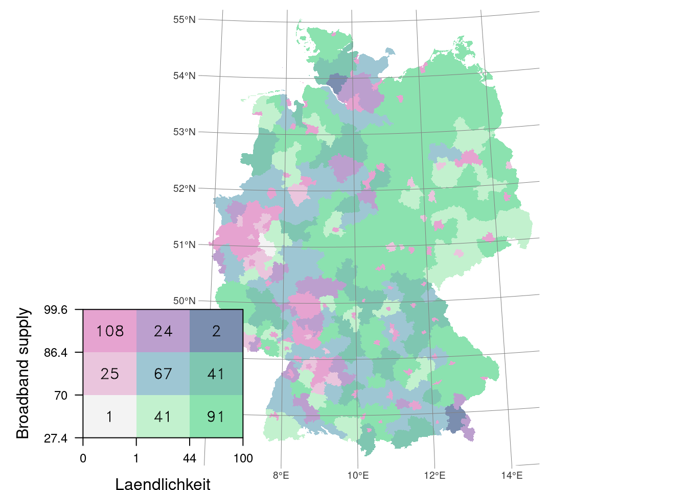
The custom script creates three quantile classes for both variables and multiplied them into nine in total. The map then is a combination of a tmap object for the map and a levelplot for the legend.
There is no documentation on the custom function create_bivar_map and its parameters. The following explains in brief every parameter:
crs_prj: projection of the map, will be passed to thetm_shapecommand of tmapdataset: name of dataset which contains the variables and geometriesx: character reference to the first variabley: character reference to the second variablex_label: label of the first variable, displayed in the legendy_label: label of the second variable, displayed in the legendcol.rmp: color ramp, to be used to symbolize the 9 classesiva.method: method to create the three classes per variablefntsize: font size, to control the label sizevp: position and width / height of the legend within the map