Chapter 3 Non-Spatial Data
How to use this book inside RStudio:
- Open a new empty R Markdown file inside RStudio
- Make sure to download the datasets used in chapter. Look out for links in the text.
- Get the path right!
- Copy either single code chunks and run it inside R (as R Markdown or R Script)
- Click on the edit button (top of the page, fourth symbol from the left) to get to the chapters source which you then can copy as a whole and paste into your R Markdown file.
The dataset we use for this introduction to non spatial data exploration and wrangling comes from the Armed Conflict Location and Event Data Project (ACLED) (Raleigh et al., 2010). ACLED is a non-governmental organization that produces event data on conflicts worldwide. It provides aggregated data at the provincial and country level, but also disaggregated point locations on events. In this chapter we will look at the curated regional Africa product. Downloaded from here: https://acleddata.com/curated-data-files/. If you are interested in other products, you can register and generate an API key free of charge. The dataset contains information on time and date of the event, actors, addressees, measures or actions, fatalities, sources, comments.
You may be familiar with the Heidelberg Institute for International Conflict Research, which works in the same area of political conflict and violence, but publishes its findings once a year in text form and as aggregated maps.
3.1 Loading data into R
From the download on the ACLED website we get a .xlsx file: Africa_1997-2022_Apr22.xlsx. You can download the file from this book’s repository directly here. In R there are two packages available to read xlsx files: readxl and xlsx. There is not much different in using one or the other. We go with the first.
3.1.1 Tabular data formats
The xlsx file contains only one sheet and there are no empty lines to skip. Therefore, it is not necessary to set other parameters for such cases.
Another common type of tabular data is .csv and can be loaded via the function read.csv().
The <- operator assigns values to variables. In this case the output of the function(indicated by the parentheses) read_excel() to the variable acled_africa. Most other programming languages use = instead. In R both operators are available but with slightly different applications.
The operators <- and = assign into the environment in which they are evaluated. The operator <- can be used anywhere, whereas the operator = is only allowed at the top level (e.g., in the complete expression typed at the command prompt) or as one of the subexpressions in a braced list of expressions.
The path within the " quotes is a relative path pointing to the data.
3.1.2 JSON - attibute: value format
Less often json files are used in R, but this is also possible.
Excourse: What is the difference of tabular and key - value / attribute - value data structures again?
CSV structure:
country, 1990, 1995, 2000, 2005, 2010, 2019
"Algeria", 0.572, 0.595, 0.637, 0.685, 0.748
"Rwanda", 0.248, , 0.341, 0.413, ,
JSON structure of the same data:
[
  {
    "1990": "0.572",
    "1995": "0.595",
    "2000": "0.637",
    "2005": "0.685",
    "2010": "0.748",
    "2019": "",
    "country": "Algeria"
  },
  {
    "1990": "0.248",
    "2000": "0.341",
    "2005": "0.413",

    "country": "Rwanda"
  }
]
With the library jsonlite JSON files can be read into R and represented as Data frames. The following chunk reads in a json file on HDI estimates downloaded from UNDP. You can download the dataset yourselve here
library(jsonlite)
hdi <- fromJSON("data/hdi.json") # read in JSON file as dataframe
head(hdi) # show first 10 lines of the dataframe
## 1990 1991 1992 1993 1994 1995 1996 1997 1998 1999 2000 2001 2002
## 1 0.302 0.307 0.316 0.312 0.307 0.331 0.335 0.339 0.344 0.348 0.35 0.353 0.384
## 2 0.65 0.631 0.615 0.618 0.624 0.637 0.646 0.645 0.655 0.665 0.671 0.678 0.684
## 3 0.572 0.576 0.582 0.586 0.59 0.595 0.602 0.611 0.621 0.629 0.637 0.647 0.657
## 4 <NA> <NA> <NA> <NA> <NA> <NA> <NA> <NA> <NA> <NA> 0.813 0.815 0.82
## 5 <NA> <NA> <NA> <NA> <NA> <NA> <NA> <NA> <NA> 0.391 0.4 0.41 0.426
## 6 <NA> <NA> <NA> <NA> <NA> <NA> <NA> <NA> <NA> <NA> <NA> <NA> <NA>
## 2003 2004 2005 2006 2007 2008 2009 2010 2011 2012 2013 2014 2015
## 1 0.393 0.409 0.418 0.429 0.447 0.447 0.46 0.472 0.477 0.489 0.496 0.5 0.5
## 2 0.691 0.696 0.706 0.713 0.722 0.728 0.733 0.745 0.764 0.775 0.782 0.787 0.788
## 3 0.667 0.677 0.685 0.69 0.7 0.702 0.711 0.721 0.728 0.728 0.729 0.736 0.74
## 4 0.827 0.833 0.827 0.837 0.837 0.84 0.839 0.837 0.836 0.858 0.856 0.863 0.862
## 5 0.435 0.446 0.46 0.473 0.489 0.501 0.515 0.517 0.533 0.544 0.555 0.565 0.572
## 6 <NA> <NA> 0.764 0.771 0.776 0.774 0.767 0.763 0.755 0.759 0.76 0.76 0.762
## 2016 2017 2018 2019 HDI Rank Country
## 1 0.502 0.506 0.509 0.511 169 Afghanistan
## 2 0.788 0.79 0.792 0.795 69 Albania
## 3 0.743 0.745 0.746 0.748 91 Algeria
## 4 0.866 0.863 0.867 0.868 36 Andorra
## 5 0.578 0.582 0.582 0.581 148 Angola
## 6 0.765 0.768 0.772 0.778 78 Antigua and Barbuda3.1.3 Binary R specific data formats
There are other, more R specific file formats like .RData and .rds. Both are binary, meaning they are encoded and not human readable. The files are also compressed which brings the advantage of a smaller file size. These formats are only readable with R.
These formats are well suited for storing intermediate results from R workflows. For example, after a computational or time intensive part of the workflow.
save/load a single object/variable
# serialize/save object names variable
saveRDS(variable, file = "path/to/file.rds")
# load saved object
readRDS(file = "path/to/file.rds")
# variable will use same name as it was saved,
# if a variable with the same name exists,
# it will be overwritten

myNewVariable <- readRDS(file = "path/to/file.rds")
# can also be assigned directly to a specific variable name
save/load multiple objects/variables
save(variable1, variable2, file = "path/to/file.RData")
load(file = "path/to/file.RData")
3.2 Understanding R data structures
Execution of the code chunks before creates entries in the Environment tab. Every variable or object we assign within a R session will be listed there. Some we inspect further like lists or data frames. Others are more complex and only brief description can be printed.
3.2.1 Assessing R object types
With the following command you can check which type an R object has. This is especially important if you try to execute a type-specific function but it does not work. One of many possibilities, but probably the easiest to fix, is that the object type does not match the one the function asks for. A simple example is trying to build the average for a list of character objects.
So with class() we can verify the object type.
## [1] "data.frame"## [1] "function"## [1] "numeric"## [1] "character"## [1] "tbl_df" "tbl" "data.frame"The object hdi is of type data.frame. It is the standard object type for tabular data in R. Comparable to a pandas dataframe in Python. It is organised in rows and columns. Whereas the rows represent observations and columns attributes. A tibble is the modern form of a data.frame. A tibble will only print the first 10 records and the data type of the columns to the console. It is also visible how many attributes/columns and records/rows the data contains. This is also observable in the Environment tab. With the following commands this can be checked directly in the console:
3.2.2 Assessing R data types
## [1] 189 32## [1] 277825 29## [1] 277825## [1] 29The ACLED dataset contains 277825 observations. In the case of ACLED, an observation is a political event. Each event has 29 attributes (given no NAs). What attributes does the dataset provide, and what types are they?
The next command prints all attributes names. Then a single column/attribute’s type is printed. The subsequent command applies the same function for retrieving the column’s type on all columns in the tibble.
## [1] "double"## ISO EVENT_ID_CNTY EVENT_ID_NO_CNTY EVENT_DATE
## "double" "character" "double" "double"
## YEAR TIME_PRECISION EVENT_TYPE SUB_EVENT_TYPE
## "double" "double" "character" "character"
## ACTOR1 ASSOC_ACTOR_1 INTER1 ACTOR2
## "character" "character" "double" "character"
## ASSOC_ACTOR_2 INTER2 INTERACTION REGION
## "character" "double" "double" "character"
## COUNTRY ADMIN1 ADMIN2 ADMIN3
## "character" "character" "character" "logical"
## LOCATION LATITUDE LONGITUDE GEO_PRECISION
## "character" "double" "double" "double"
## SOURCE SOURCE_SCALE NOTES FATALITIES
## "character" "character" "character" "double"
## TIMESTAMP
## "double"Some of the data types might be familiar from other programming languages or software applications. What if we apply the same function on the R objects we inspected three chunks earlier.
## [1] "list"## [1] "closure"## [1] "double"## [1] "character"## [1] "list"1 is of class numeric, but of type double. Tibble and data frame actually are lists. Brief background is that a data frame is a more complex two-dimensonal object structure that is built upon the list type.
3.3 Exploring data
3.3.1 handle data frames
Columns of data frames and tibbles can be either selected via their name and the $ operator like tibble$columnName or by index like acled_africa[<ROW>,<COLUMN>] were <ROW> is the positional index of the row and <COLUMN> the positional index of the column.
- With
acled_africa[1,]the first row and all columns of a data frame or tibble will be selected. - With
acled_africa[,1]the first column and all rows of a data frame or tibble will be selected. - With
acled_africa[4,20]the fourth row and the 20th column are selected only. So basically a single cell / value.
## # A tibble: 1 × 29
##     ISO EVENT_ID_CNTY EVENT_ID_NO_CNTY EVENT_DATE           YEAR TIME_PRECISION
##   <dbl> <chr>                    <dbl> <dttm>              <dbl>          <dbl>
## 1    12 ALG1                         1 1997-01-01 00:00:00  1997              1
## # ℹ 23 more variables: EVENT_TYPE <chr>, SUB_EVENT_TYPE <chr>, ACTOR1 <chr>,
## #   ASSOC_ACTOR_1 <chr>, INTER1 <dbl>, ACTOR2 <chr>, ASSOC_ACTOR_2 <chr>,
## #   INTER2 <dbl>, INTERACTION <dbl>, REGION <chr>, COUNTRY <chr>, ADMIN1 <chr>,
## #   ADMIN2 <chr>, ADMIN3 <lgl>, LOCATION <chr>, LATITUDE <dbl>,
## #   LONGITUDE <dbl>, GEO_PRECISION <dbl>, SOURCE <chr>, SOURCE_SCALE <chr>,
## # NOTES <chr>, FATALITIES <dbl>, TIMESTAMP <dbl>## # A tibble: 277,825 × 1
## ACTOR1
## <chr>
## 1 GIA: Armed Islamic Group
## 2 GIA: Armed Islamic Group
## 3 GIA: Armed Islamic Group
## 4 GIA: Armed Islamic Group
## 5 GIA: Armed Islamic Group
## 6 GIA: Armed Islamic Group
## 7 Police Forces of Algeria (1994-1999)
## 8 GIA: Armed Islamic Group
## 9 GIA: Armed Islamic Group
## 10 Military Forces of Algeria (1994-1999)
## # ℹ 277,815 more rows## # A tibble: 1 × 1
## EVENT_DATE
## <dttm>
## 1 1997-01-16 00:00:00Another, more convenient way to check out a dataset’s attributes is the summary() function
##       ISO        EVENT_ID_CNTY      EVENT_ID_NO_CNTY
##  Min.   : 12.0   Length:277825      Min.   :    1
##  1st Qu.:231.0   Class :character   1st Qu.: 2020
##  Median :566.0   Mode  :character   Median : 5372
##  Mean   :510.2                      Mean   : 8028
##  3rd Qu.:710.0                      3rd Qu.:10870
##  Max.   :894.0                      Max.   :48946
##    EVENT_DATE                          YEAR      TIME_PRECISION
##  Min.   :1997-01-01 00:00:00.00   Min.   :1997   Min.   :1.000
##  1st Qu.:2012-09-29 00:00:00.00   1st Qu.:2012   1st Qu.:1.000
##  Median :2017-01-30 00:00:00.00   Median :2017   Median :1.000
##  Mean   :2015-03-13 22:19:15.33   Mean   :2015   Mean   :1.135
##  3rd Qu.:2020-04-02 00:00:00.00   3rd Qu.:2020   3rd Qu.:1.000
##  Max.   :2022-04-22 00:00:00.00   Max.   :2022   Max.   :3.000
##   EVENT_TYPE        SUB_EVENT_TYPE        ACTOR1          ASSOC_ACTOR_1
##  Length:277825      Length:277825      Length:277825      Length:277825
##  Class :character   Class :character   Class :character   Class :character
##  Mode  :character   Mode  :character   Mode  :character   Mode  :character
##
##
##
##      INTER1         ACTOR2          ASSOC_ACTOR_2          INTER2
##  Min.   :1.000   Length:277825      Length:277825      Min.   :0.000
##  1st Qu.:2.000   Class :character   Class :character   1st Qu.:0.000
##  Median :3.000   Mode  :character   Mode  :character   Median :2.000
##  Mean   :3.563                                         Mean   :3.231
##  3rd Qu.:6.000                                         3rd Qu.:7.000
##  Max.   :8.000                                         Max.   :8.000
##   INTERACTION      REGION            COUNTRY             ADMIN1
##  Min.   :10.0   Length:277825      Length:277825      Length:277825
##  1st Qu.:15.0   Class :character   Class :character   Class :character
##  Median :33.0   Mode  :character   Mode  :character   Mode  :character
##  Mean   :33.8
##  3rd Qu.:55.0
##  Max.   :88.0
##     ADMIN2           ADMIN3          LOCATION            LATITUDE
##  Length:277825      Mode:logical   Length:277825      Min.   :-34.710
##  Class :character   NA's:277825    Class :character   1st Qu.: -0.360
##  Mode  :character                  Mode  :character   Median :  6.264
##                                                       Mean   :  6.912
##                                                       3rd Qu.: 13.500
##                                                       Max.   : 37.282
##    LONGITUDE       GEO_PRECISION      SOURCE          SOURCE_SCALE
##  Min.   :-25.163   Min.   :1.000   Length:277825      Length:277825
##  1st Qu.:  9.123   1st Qu.:1.000   Class :character   Class :character
##  Median : 28.100   Median :1.000   Mode  :character   Mode  :character
##  Mean   : 22.345   Mean   :1.275
##  3rd Qu.: 33.010   3rd Qu.:1.000
##  Max.   : 63.475   Max.   :3.000
##     NOTES             FATALITIES         TIMESTAMP
##  Length:277825      Min.   :   0.000   Min.   :1.553e+09
##  Class :character   1st Qu.:   0.000   1st Qu.:1.611e+09
##  Mode  :character   Median :   0.000   Median :1.619e+09
##                     Mean   :   2.941   Mean   :1.614e+09
##                     3rd Qu.:   1.000   3rd Qu.:1.628e+09
##                     Max.   :1350.000   Max.   :1.651e+09
The summary function not only provides info on amount of observations , NA’s and datatype’s but also scales and ranges for numerical attributes.
Overview of the main attributes of interest
- YEAR: Year when an event took place
- EVENT_DATE: Exact date when an event took place
- COUNTRY: Country in which the the event took place
- ACTOR1: Political actor who commited an action
- ACTOR2: (Political) actor who is the addressee or target of an action
- EVENT_TYPE: Type of event; 6 different available
- SUB_EVENT_TYPE: Subtype of event; 25 different available
- FATALITIES: Amount of fatalities caused by the event
- LATITUDE & LONGITUDE: Both together provide a point coordiante georeference, which are not going to use in this chapter
3.3.2 Missing data
Is there any missing data in the dataset?
Missing data in R is represented as NA. With the following code we check the amount of NA’s for each column:
##              ISO    EVENT_ID_CNTY EVENT_ID_NO_CNTY       EVENT_DATE
##                0                0                0                0
##             YEAR   TIME_PRECISION       EVENT_TYPE   SUB_EVENT_TYPE
##                0                0                0                0
##           ACTOR1    ASSOC_ACTOR_1           INTER1           ACTOR2
##                0           206757                0            74458
##    ASSOC_ACTOR_2           INTER2      INTERACTION           REGION
##           225170                0                0                0
##          COUNTRY           ADMIN1           ADMIN2           ADMIN3
##                0                1             2151           277825
##         LOCATION         LATITUDE        LONGITUDE    GEO_PRECISION
##                0                0                0                0
##           SOURCE     SOURCE_SCALE            NOTES       FATALITIES
##                0                0             9288                0
##        TIMESTAMP
##                0
Every record contains a year and at least one main actor and event type.
The occurence of NA’s can have several implications for one’s analysis:
numeric_vector <- c(1,2,3,4,NA) # vector of numericals. Vector is a kind of list, but only allows to store data of the same type. Vectors are one-dimensional.
sum(numeric_vector) # well we would expect the sum to be 10, but the NA causes a problem here
## [1] NAsum(numeric_vector, na.rm = TRUE) # na.rm or na.omit are common parameters to handle NAs in the dataset## [1] 10What is the distribution of events by year?
##
##  1997  1998  1999  2000  2001  2002  2003  2004  2005  2006  2007  2008  2009
##  3209  4546  4882  4175  3611  4297  3750  3174  2909  2739  3897  5083  3863
##  2010  2011  2012  2013  2014  2015  2016  2017  2018  2019  2020  2021  2022
##  4396  8136  9793 14234 16590 16984 17308 17665 19678 25618 32661 33971 10656
year_cross_eventtype <- table(acled_africa$YEAR, acled_africa$EVENT_TYPE)
head(year_cross_eventtype)##
## Battles Explosions/Remote violence Protests Riots Strategic developments
## 1997 1184 131 244 137 615
## 1998 1650 136 249 183 1115
## 1999 2685 198 218 174 679
## 2000 1814 224 256 227 445
## 2001 1502 127 231 267 328
## 2002 1724 183 270 245 186
##
## Violence against civilians
## 1997 898
## 1998 1213
## 1999 928
## 2000 1209
## 2001 1156
## 2002 1689The table() function creates a contingency table or crosstab. It displays the frequency of a single or multiple attributes. The frequency is the sum of observations per variable or variable combination.
3.3.3 Visualization
We can also answer that by plotting the data. R has several big packages that serve plotting:
- graphics
- lattice
- ggplot2
All have their pros and cons but we will focus on ggplot2 here there possible.
Using the graphics package we can use the command hist that requires a vector of values. Other parameters can be used to specify the title or the axis label. The help file indicates possibilities for fine tuning the plot.
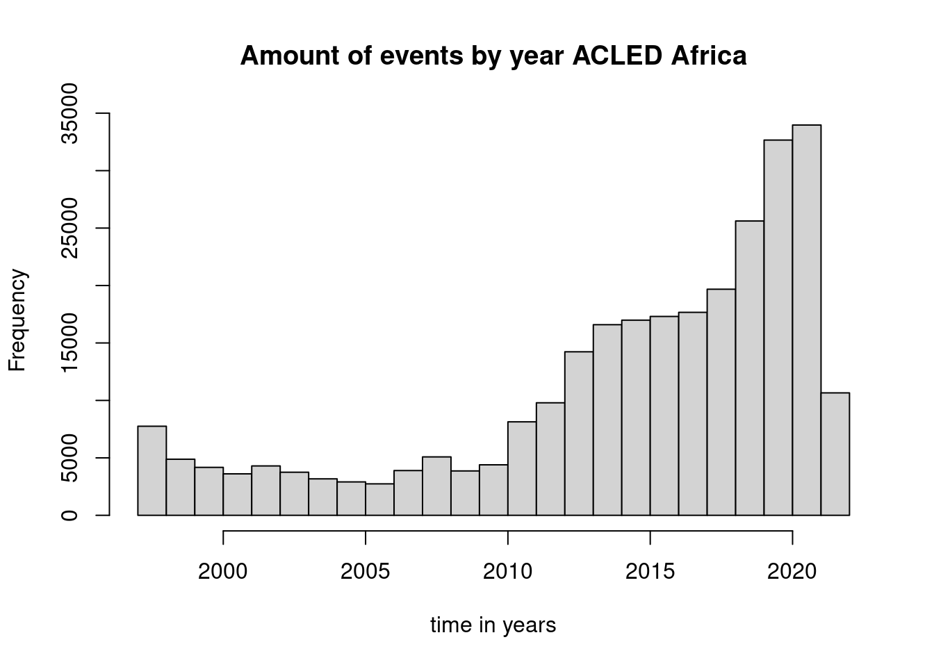
Plotting with ggplot2 follows a different syntax. We start with ggplot to define the data.frame we will be using and to map aesthetics to variables/columns of that data frame. Next we add (with a plus sign) different graphical functions that specify e.g. the type of plot to be used. In the following example we distinguish the different event types, by stacking histograms for each event type.
library(ggplot2)

ggplot(data = acled_africa, mapping = aes(x=YEAR, fill=EVENT_TYPE)) +
  geom_histogram(bins=24) +
  xlab("")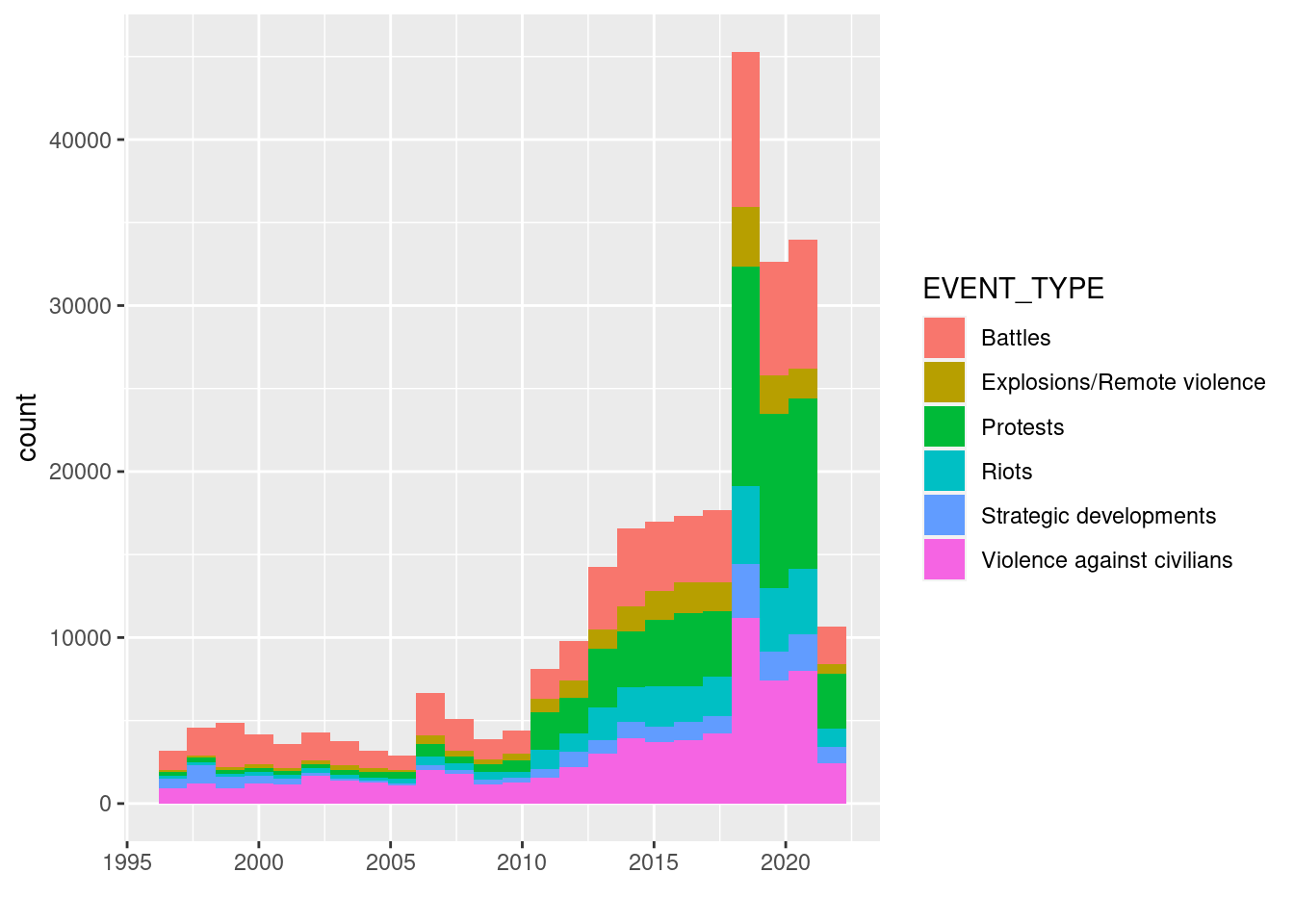
First the ggplot() function is called and the variables of interest are configured in the aesthetics parameter. With a + (!) operator subsequent ggplot functions are added to the plot. The pipe does not work here. The next ggplot function is a layer that specifies the type of plot, e.g. geom_point, geom_line, geom_bar or geom_tile. Other ggplot functions that can be added optionally are to configure scales, labeling, legend, the theme or facet options.
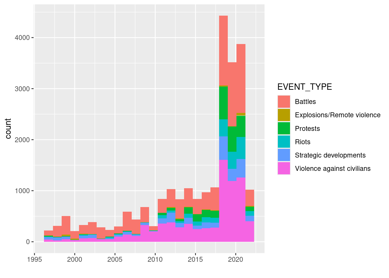
But What do we see in the plot? A sharp increase in 2019 is visible. What does this look like for a single country, e.g. Democratic Republic of Congo:
##
## Attaching package: 'dplyr'
## The following objects are masked from 'package:stats':
##
## filter, lag## The following objects are masked from 'package:base':
##
## intersect, setdiff, setequal, uniondrc_subset <- acled_africa |> filter(COUNTRY=="Democratic Republic of Congo")
ggplot(drc_subset, aes(x=YEAR)) +
geom_histogram(bins=24) + xlab("")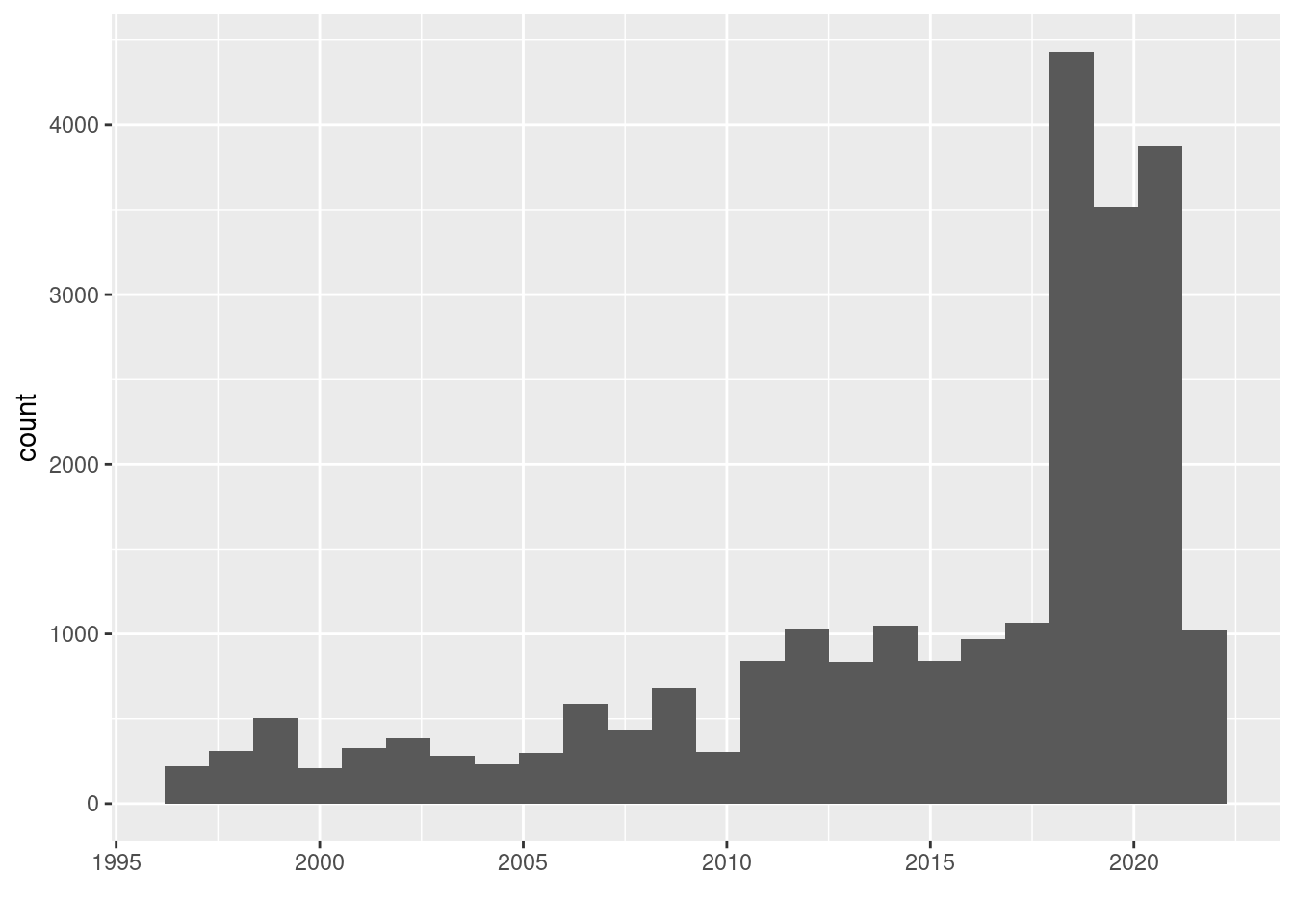
More ressources on ggplot here: * ggplot2 essentials (sthda.com) * The R Graph Gallery (r-graph-gallery.com)
3.3.4 Subsetting
dplyr is the Swiss army knife package for data wrangling and manipulation. The filter function comes with it. The == operator corresponds to exactly equal. Only rows that meet these criteria in the selected columns are evaluated as true and returned.
Selection of other logical operators:
| Operator | Description |
|---|---|
| != | not equal |
| > | greater than |
| < | less than |
| >= | greater than or equal to |
| <= | less than or equal to |
| a & b | logical AND: a AND b |
| a | b | logical OR: a OR b |
| a %in% b | comparing two sequences / columns |
| is.na(a) | test if a is NA |
The |> operator is the so-called pipe. The pipe operator is a way to avoid the nesting of functions and to store intermediate steps.
This becomes more clear with longer chains of commands. It works by piping the outcome of the function before the pipe as the first argument into the function after the pipe operator. Before R version 4.0 the |> pipe was not part of base R, the basic functionality provided by R without any extending libraries / packages. But there was the magrittr pipe %>%. The magrittr pipe is still very popular and you will see usage of it in a lot of documentation and tutorials. The functionality between |> and %>% is the same. However in roder to use the magrittr pipe you either have to load the library with library(magrittr) or a library that uses magrittr via dependencies like dplyr, tidyr or tidyverse. In RStudio you can use the hotkey combination [ctrl] + [shift] + [m] to faster write pipes. Out of the box, RStudio will use the magrittr pipe, in the settings however you can change it to the native pipe.
# sequentiell with individua assignment
numeric_vectrs <- c(1,2,3,4)
mean_vectrs <- mean(numeric_vectrs)
mean_string <- as.character(mean_vectrs)
paste0(mean_string, " is the mean")
## [1] "2.5 is the mean"# nested
paste( # function to combine character data types to one
as.character( # function to convert data type to character type
mean( # function to calculate the average of a vector, list, sequence of numeric data types
c(1,2,3,4) # a vector of numerics
)
)
," is the mean") # second input for the concatenate function## [1] "2.5 is the mean"## [1] "2.5 is the mean"## [1] "2.5 is the mean"Back to the ACLED dataset.
- How many events with the event type Violence against civilians took place since 2020 in DRC.
# Counts the number of rows that meet filter criteria.
drc_subset |>
  filter(EVENT_TYPE == "Violence against civilians" & YEAR > 2020) |>
  count()
## # A tibble: 1 × 1
## n
## <int>
## 1 1661- How many fatalities have occurred in events of the violence against civilians type since 2020?
# Sums up the number of fatalities of each row that meets the filter criteria.
drc_subset |>
  filter(EVENT_TYPE == "Violence against civilians" & YEAR > 2020) |>
  summarise(total_fatalities=sum(FATALITIES))
## # A tibble: 1 × 1
## total_fatalities
## <dbl>
## 1 31093.3.5 Transform
- Who is the actor in DRC that perpetuated the most events of the type Violence against civilians since 2020, how does it compare to Uganda?
DRC:
drc_subset |>
  filter(EVENT_TYPE == "Violence against civilians" & YEAR > 2020) |>
  group_by(ACTOR1) |>
  summarise(violent_acts=n()) |>
  arrange(desc(violent_acts))
## # A tibble: 107 × 2
## ACTOR1 violent_acts
## <chr> <int>
## 1 Unidentified Armed Group (Democratic Republic of Congo) 578
## 2 ADF: Allied Democratic Forces 372
## 3 CODECO-URDPC: Cooperative for Development of Congo (Union of Re… 109
## 4 CODECO: Cooperative for Development of Congo 79
## 5 Military Forces of the Democratic Republic of Congo (2019-) 64
## 6 Mayi Mayi Militia 39
## 7 FPAC: Ituri Self-Defense Popular Front (Zaire) 26
## 8 Batwa Ethnic Militia (Democratic Republic of Congo) 24
## 9 Police Forces of the Democratic Republic of Congo (2019-) 22
## 10 Chini Ya Kilima-FPIC: Patriotic and Integrationist Force of Con… 15
## # ℹ 97 more rowsUganda:
acled_africa |>
  filter(EVENT_TYPE == "Violence against civilians" & YEAR > 2020 & COUNTRY=="Uganda") |>
  group_by(ACTOR1) |>
  summarise(violent_acts=n()) |>
  arrange(desc(violent_acts))
## # A tibble: 31 × 2
## ACTOR1 violent_acts
## <chr> <int>
## 1 Unidentified Armed Group (Uganda) 88
## 2 Police Forces of Uganda (1986-) 80
## 3 Military Forces of Uganda (1986-) 43
## 4 Karamajong Ethnic Militia (Uganda) 35
## 5 Military Forces of Uganda (1986-) Local Defense Unit 8
## 6 Private Security Forces (Uganda) 8
## 7 Police Forces of Uganda (1986-) Prison Guards 7
## 8 Dodoth Ethnic Militia (Uganda) 3
## 9 Unidentified Communal Militia (Uganda) 3
## 10 Unidentified Ethnic Militia (Uganda) 3
## # ℹ 21 more rowsThe group_by() function is used to create groups within the tibble. Subsequent functions on the tibble, like summarizing in the example are executed on the groups instead on the whole table.
n() is a context dependent expression that returns the current group size, comparable to count().
arrange sorts the tibble based on one or multiple columns. The order type is ascending by default. With desc() it is changed to descending.
Selection of other summary functions:
| Function | description |
|---|---|
| mean() | mean or average |
| median() | median |
| min() | minimum value |
| max() | maximum value |
| quantile() | nth quantile |
| sd() | standard deviation |
| var() | variance |
| first() | first value |
| last() | last value |
What are the top 10 countries with respect to amount of events?
## # A tibble: 57 × 2
##    COUNTRY                      event_count
##    <chr>                              <int>
##  1 Somalia                            36352
##  2 Democratic Republic of Congo       24249
##  3 Nigeria                            24193
##  4 Sudan                              16857
##  5 South Africa                       16476
##  6 Algeria                            11875
##  7 Egypt                              11300
##  8 Libya                              10905
##  9 Burundi                             9767
## 10 Tunisia                             9228
## # ℹ 47 more rows
What are the top 10 countries for the last 5 years with respect to all event types?
acled_africa |>
  filter(YEAR > 2017) |>
  group_by(COUNTRY) |>
  summarize(event_count=n()) |>
  arrange(desc(event_count))
## # A tibble: 57 × 2
## COUNTRY event_count
## <chr> <int>
## 1 Democratic Republic of Congo 12837
## 2 Nigeria 12797
## 3 Somalia 11662
## 4 South Africa 7052
## 5 Algeria 7017
## 6 Sudan 5833
## 7 Tunisia 5616
## 8 Burkina Faso 4981
## 9 Cameroon 4726
## 10 Mali 4699
## # ℹ 47 more rows3.4 Modifying data
Next we will alter the tibble according to our needs. First we will add a new column with simplified event types. We reduce the number of columns to the ones we are interested in. Then we pivot the table from the current long to the wide format. We define this format as one record/row being unique by country and year.
acled_africa_altered <- acled_africa |>
  mutate(event_type_simple = case_when(
    EVENT_TYPE == "Battles"~ "battles",
    EVENT_TYPE == "Explosions/Remote violence"  ~ "remote_violence",
    EVENT_TYPE == "Protests" ~ "protests",
    EVENT_TYPE == "Riots" ~ "riots",
    EVENT_TYPE == "Strategic developments" ~ "strategic_dev",
    EVENT_TYPE == "Violence against civilians" ~ "violence_civilians",
  )) |>
  select(YEAR, COUNTRY, event_type_simple) # the first attribute contains information on the country code
With the mutate() function of the dplyr library, one can modify existing columns or add new ones.
In combination with the case_when() it is possible to fill a column based on conditions. Take a look into this blogpost for further information. The select() function extracts specified columns into a new tibble. Inversely, certain columns can also be excluded using the following syntax: select(-c(columnA, columnB, columnC))
Next we aggregate the tibble by event type.
aggregated_events <- acled_africa_altered |>
  group_by(COUNTRY, YEAR, event_type_simple) |>
  summarize(event_count=n())
## `summarise()` has grouped output by 'COUNTRY', 'YEAR'. You can override using
## the `.groups` argument.The resulting tibble is ~6590 rows long. We want a tibble were each country and year combination define a single row. For this we need to pivot the table from the long format to the wide one.
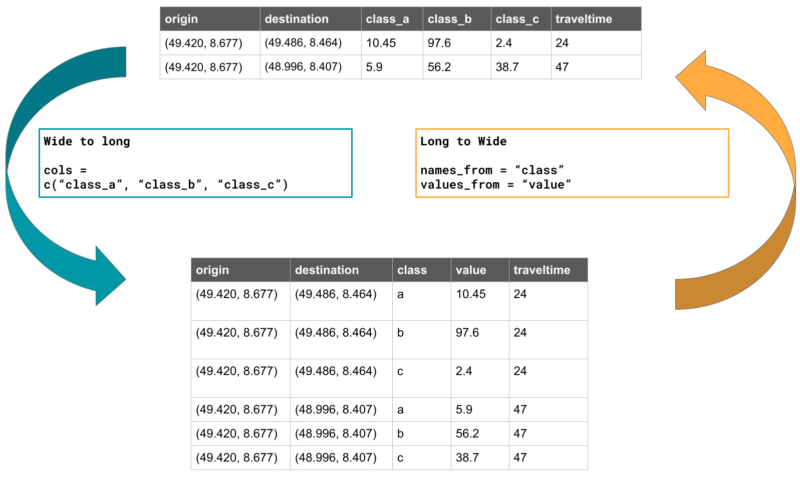
(#fig:pivot_img)Example on pivoting a table from wide to long and long to wide format
##
## Attaching package: 'tidyr'
## The following object is masked from 'package:magrittr':
##
## extractaggregated_events_wide <- aggregated_events |>
ungroup() |> # the tibble still contains grouping information from group_by, this function removes it.
pivot_wider(names_from=event_type_simple, values_from=event_count)
aggregated_events_wide## # A tibble: 1,269 × 8
## COUNTRY YEAR battles remote_violence violence_civilians protests
## <chr> <dbl> <int> <int> <int> <int>
## 1 Algeria 1997 8 17 116 NA
## 2 Algeria 1998 14 13 20 1
## 3 Algeria 1999 27 11 25 NA
## 4 Algeria 2000 95 12 61 2
## 5 Algeria 2001 78 11 48 18
## 6 Algeria 2002 99 37 72 12
## 7 Algeria 2003 91 18 45 28
## 8 Algeria 2004 52 14 22 12
## 9 Algeria 2005 50 18 10 6
## 10 Algeria 2006 98 48 32 7
## # ℹ 1,259 more rows
## # ℹ 2 more variables: strategic_dev <int>, riots <int>aggregated_events_wide <- aggregated_events_wide |>
rowwise() |> # if not set to rowwise, whole columns will be summed up.
mutate(total = sum(battles, remote_violence, violence_civilians, protests, strategic_dev, riots, na.rm=TRUE)) # the parameter na.rm=T, will ignore NAs, otherwise a single NA in the column selection will cause the result to be NA too.The tibble is now reduced to 1269 rows. With pivot_longer() the same process vice versa can be done.
Next we add a column on the cumulative sum of the total events by country and year.
aggregated_events_wide <- aggregated_events_wide |>
  group_by(COUNTRY) |>
  arrange(YEAR) |>
  mutate(cum_total = cumsum(total)) |>
  ungroup() |>
  arrange(COUNTRY,YEAR)
aggregated_events_wide
## # A tibble: 1,269 × 10
## COUNTRY YEAR battles remote_violence violence_civilians protests
## <chr> <dbl> <int> <int> <int> <int>
## 1 Algeria 1997 8 17 116 NA
## 2 Algeria 1998 14 13 20 1
## 3 Algeria 1999 27 11 25 NA
## 4 Algeria 2000 95 12 61 2
## 5 Algeria 2001 78 11 48 18
## 6 Algeria 2002 99 37 72 12
## 7 Algeria 2003 91 18 45 28
## 8 Algeria 2004 52 14 22 12
## 9 Algeria 2005 50 18 10 6
## 10 Algeria 2006 98 48 32 7
## # ℹ 1,259 more rows
## # ℹ 4 more variables: strategic_dev <int>, riots <int>, total <int>,
## # cum_total <int>Lastly we plot the totals by country as facet plot.
aggregated_events_wide |>
  ggplot(aes(x=YEAR, y=total)) +
  geom_line(alpha=0.5) +
  facet_wrap(~COUNTRY, ncol = 6)
## `geom_line()`: Each group consists of only one observation.
## ℹ Do you need to adjust the group aesthetic?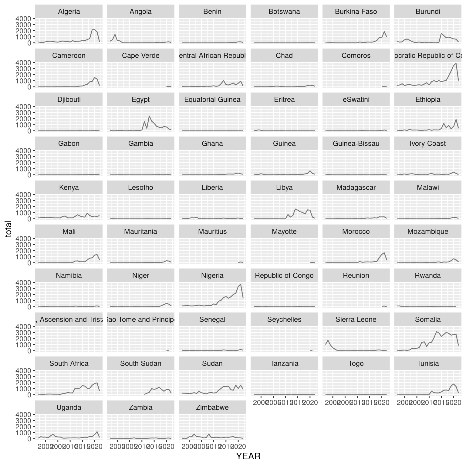
With the facet wrap function of ggplot, facet plots can be created out of attributes that define groups within the data.
Now we join the hdi data per country and year
##  [1] "1990"     "1991"     "1992"     "1993"     "1994"     "1995"
##  [7] "1996"     "1997"     "1998"     "1999"     "2000"     "2001"
## [13] "2002"     "2003"     "2004"     "2005"     "2006"     "2007"
## [19] "2008"     "2009"     "2010"     "2011"     "2012"     "2013"
## [25] "2014"     "2015"     "2016"     "2017"     "2018"     "2019"
## [31] "HDI Rank" "Country"## [1] "1990" "1991" "1992" "1993" "1994" "1995" "1996" "1997" "1998" "1999"
## [11] "2000" "2001" "2002" "2003" "2004" "2005" "2006" "2007" "2008" "2009"
## [21] "2010" "2011" "2012" "2013" "2014" "2015" "2016" "2017" "2018" "2019"hdi_long <- hdi |>
pivot_longer(cols=all_of(year_cols), names_to = "year", values_to = "hdi") # all_of() is necessary that the pivot_longer function reads year_cols vector not as the character vector it is, but to select the column by the names
# check attributes to be used for joining
names(aggregated_events_wide)## [1] "COUNTRY" "YEAR" "battles"
## [4] "remote_violence" "violence_civilians" "protests"
## [7] "strategic_dev" "riots" "total"
## [10] "cum_total"## [1] "HDI Rank" "Country" "year" "hdi"## [1] "character"## [1] "character"## [1] "double"## [1] "character"hdi_long$year <- as.numeric(hdi_long$year) # change character column to numeric
typeof(hdi_long$year) # woroked## [1] "double"aggregated_events_wide_hdi <- aggregated_events_wide |>
left_join(hdi_long, by=c("COUNTRY"="Country", "YEAR"="year"))
aggregated_events_wide_hdi## # A tibble: 1,269 × 12
## COUNTRY YEAR battles remote_violence violence_civilians protests
## <chr> <dbl> <int> <int> <int> <int>
## 1 Algeria 1997 8 17 116 NA
## 2 Algeria 1998 14 13 20 1
## 3 Algeria 1999 27 11 25 NA
## 4 Algeria 2000 95 12 61 2
## 5 Algeria 2001 78 11 48 18
## 6 Algeria 2002 99 37 72 12
## 7 Algeria 2003 91 18 45 28
## 8 Algeria 2004 52 14 22 12
## 9 Algeria 2005 50 18 10 6
## 10 Algeria 2006 98 48 32 7
## # ℹ 1,259 more rows
## # ℹ 6 more variables: strategic_dev <int>, riots <int>, total <int>,
## # cum_total <int>, `HDI Rank` <chr>, hdi <chr>3.5 Analyzing data
We load timeseries data on population, GDP per capita and life expectancy from gapminder. Gapminder is a dataset facilitated by the Gapminder foundation. Driving force behind the project was Hans Rosling, the author of the book Factfulness. You can download the data here
gapminder <- read.csv("data/gapminder.csv") |>
  tibble() # read.csv loads data as data.frame, with pipe and tibble function we get a tibble directly.
The gapminder dataset is a csv, we use the function read.csv to load it. We don’t need to alter the parameters, as the csv is completely compliant with the csv standard’s default. If you use csv’s that for instance were compiled by a german authority, it can well be that you need to adjust parameters on string escaping and the delimiter.
The dataset contains the following attributes:
- country: country name
- continent: continent name
- year: year of measurement, ranges from 1952 to 2007
- life expectancy at birth, in years
- pop: population
- gdpPercap: (GDP per capita (US$, inflation-adjusted))
Next we create some plots on life expectancy by continent. Comparison of the years 1997 and 2007 in terms of life expectancy x GDP. Can we predict life expectancy from GDP with a linear model?
gapminder |>
  ggplot(aes(x=year, y=lifeExp, group=country)) +
  geom_line(alpha=0.5) +
  xlab("") +
  facet_wrap(~continent)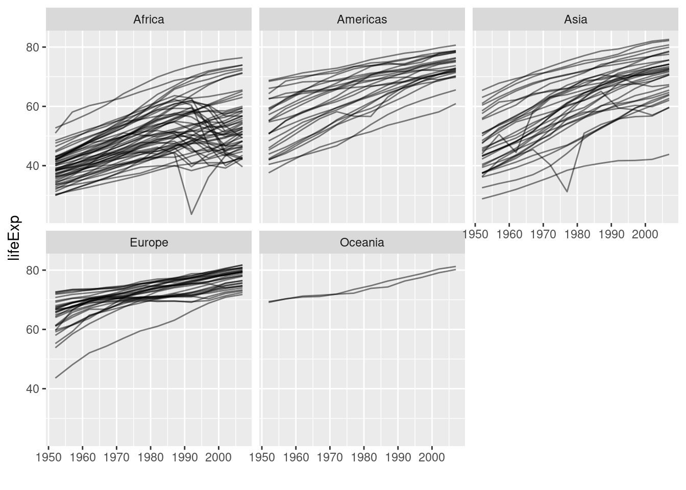
g_subset <- gapminder |>
  filter (year==1997 | year==2007)

g_subset |>
#  filter (year==2007) |>
  ggplot(aes(x=gdpPercap, y=lifeExp, color=country, size=pop)) +
  geom_point() +
  facet_wrap(~year) +
  xlab("GDP per capita [interntational US$]") +
  ylab("Life expectancy [years]") +
  theme(legend.position = "none")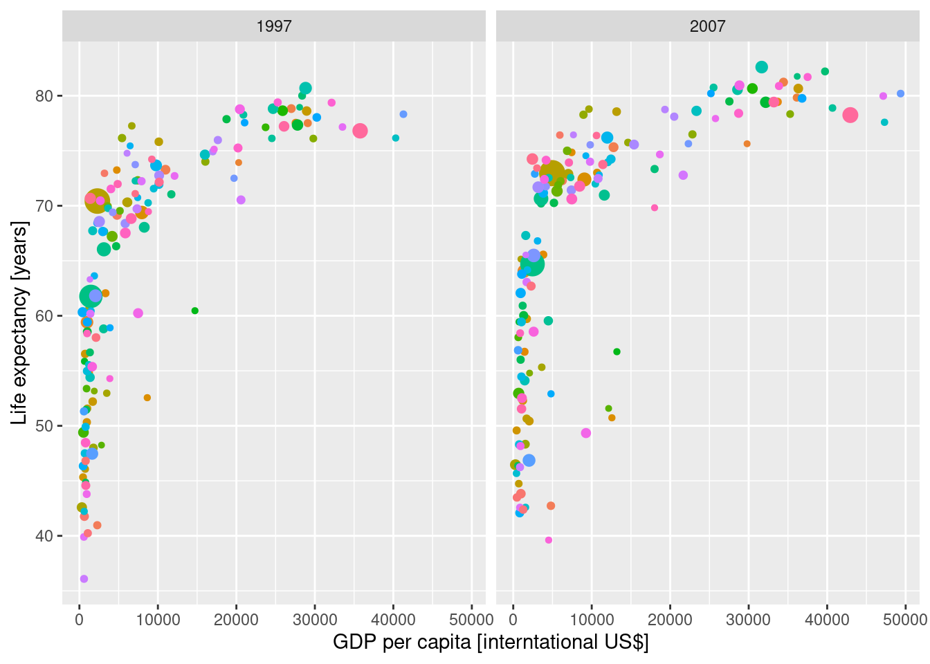
gapminder |>
  filter(continent=="Africa") |>
  ggplot(aes(x=lifeExp, y=gdpPercap)) +
  geom_point() + xlab("GDP per capita [interntational US$]") +
ylab("Life expectancy [years]") 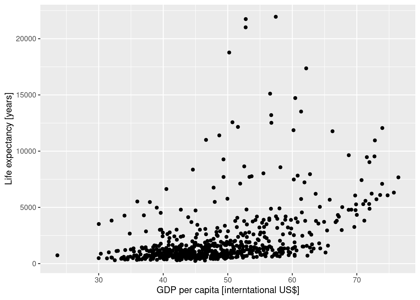
gapminder |>
  filter(continent=="Africa") |>
  ggplot(aes(x=lifeExp, y=gdpPercap)) +
  geom_point() +
  geom_smooth(method=lm) + xlab("GDP per capita [interntational US$]") +
  ylab("Life expectancy [years]") +
  theme_light()
## `geom_smooth()` using formula = 'y ~ x'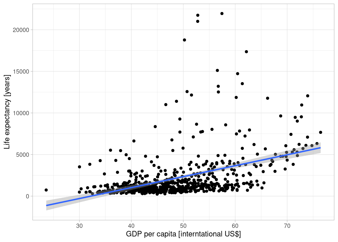
Next we create a linear model with the gapminder dataset. The dependent variable is life expectancy. GPD per capita is the predictor. In R the syntax follows this pattern:
[dependent variable] ~ [predictor A] + [predictor B] + [predictor C]
If there are NAs in the dataset, you need to set the na.action parameter accordingly.
##
## Call:
## lm(formula = lifeExp ~ gdpPercap, data = gapminder)
##
## Residuals:
##     Min      1Q  Median      3Q     Max
## -82.754  -7.758   2.176   8.225  18.426
##
## Coefficients:
##              Estimate Std. Error t value Pr(>|t|)
## (Intercept) 5.396e+01  3.150e-01  171.29   <2e-16 ***
## gdpPercap   7.649e-04  2.579e-05   29.66   <2e-16 ***
## ---
## Signif. codes:  0 '***' 0.001 '**' 0.01 '*' 0.05 '.' 0.1 ' ' 1
##
## Residual standard error: 10.49 on 1702 degrees of freedom
## Multiple R-squared:  0.3407, Adjusted R-squared:  0.3403
## F-statistic: 879.6 on 1 and 1702 DF,  p-value: < 2.2e-16
The estimated effect of our predictor GDP per capita is significantly different from zero, this can be seen by comparing the standard error with the regression coefficient estimate or by looking at the associated p-value.
The model explains 34% of the variance, which is depicted as R-square. Which clearly indicates that there is a clear relationship but that there are presumably other factors that explain the variability of the data.
If the GDP per capita increases by 1000 US$ (purchasing power adjusted), the life expectancy increases on average by 7.649.
(The linear model has several shortcommings and could be improved in various ways (temporal auto.correlation, prediction of life expectancy below zero,…) but this is not the point here.)