Chapter 8 Bivariate relationships considering spatial pattern

Correlation coefficients are a well known measure of association between variables. The question is how these can or should be modified if we apply them to spatialy structured data. here we focus on association between numerical scaled variables and ignore association measures for ordinal or nominal variables.

8.1 Cheat sheet

The following packages are required for this chapter:

require(sf)
require(spdep)
require(sp)
require(ncf)
require(tmap)
require(ggplot2)
require(ggpubr)
require(gstat) # for simulation of autocorrelated data
require(dplyr)
require(SpatialPack) # for the modified t-test

Important commands:

• spdep::lee.mc - permutation test for Lee’s L
• spdep::lag.listw - computing a spatially lagged version of a variable vector
• cor.test - Pearson’s r with test

8.2 Adjusted t-test

8.3 Motivation

In presence of positive spatial autocorrelation our effective sample size is smaller than the sample size. This is due to shared information between observations. The normal t-test for Pearson’s r is therefore incorrect.

The simplest solution is to calculate the effective sample size under consideration of spatial autocorrelation.

The effective sample size \(n'\) in absence of autocorrelation: \(n' = n\) (number of observations). In presence of autocorrelation this needs to be modified to

\[n'= \frac{n^2}{\sum_{i=1}^n\sum_{j=1}^nCor(x_i, y_i)}\]

The exact formula depends on the from of the correlation function. For a first order autoregressive correlation structure (\(Cor(x_i, x_j)= \rho^{|i-j}\)):

\[n'=(1+2\frac{\rho}{1-\rho}(1-\frac{1}{n})-2\frac{\rho^2}{(1-\rho)^2} \frac{1-\rho^{n-1}}{n}) \cdot n\]

This can be simplified for large n:

\[n' \cong n \frac{1-\rho}{1+\rho}\]

# function to calculate the effective sampel size for large n and the simple first order autoregresive function
neff <- function(n, rho)
{
  res <- n*(1-rho)/(1+rho)
  return(res)
}

• e.g. \(n=1000\) and \(\rho = 0.7\) \(\rightarrow n' =\) 176.4705882
• e.g. \(n=1000\) and \(\rho = 0.9\) \(\rightarrow n' =\) 52.6315789

The modified t-test by Clifford and Richardson (Clifford et al. (1989) and Dutilleul et al. (1993)) uses the covariance for all observations in a distance band as a measure to capture spatial autocorrelation (cf. correlogram). The function is available as spatialPack::modified.ttest.

8.4 Bivariate Moran’s I

Bivariate Moran’s I is a measure of autocorrelation of X with the spatial lag of Y. As such, the resultant measure may overestimate the amount of spatial autocorrelation which may be a product of the inherent correlation of X and Y.

\[I_B = \frac{\sum_i(\sum_j w_{i,j}y_j\cdot x_i)}{\sum_i x_i^2}\] It only captures autocorrelation of one variable and completely ignores the spatial pattern of the second variable. \(I_{X,Y}\) might be different from \(I_{Y,X}\) which might provide an obstacle for interpretation. On the other hand, the bivariate Moran’s I looks at the relationship from a directed perspective - \(x\) depends on the lag of \(y\) - that might be interesting for spatial modelling.

Using the spatial lag operator this can be written as:

\[I_{X,Y} = \frac{\sum_i(x_i-\bar{x})(\tilde{y}-\bar{y})}{\sqrt{\sum_i(x_i-\bar{x})^2} \sqrt{\sum_i(y_i-\bar{y})^2}} \cong \sqrt{SSS_Y} \cdot r_{x,\tilde{y}}\]

8.5 Lee’s L - measuring association between spatially autocorrelated variables

Spatial autocorrelation also influences the correlation between variables. Using the standard Pearson correlation coefficient ignores the fact that part of the association originates from the spatial autocorrelation of the two variables. Lee (2001) developed an index to measure the bivariate spatial association by a fusion of Pearson’s correlation coefficient and Moran’s I. More precisely, Moran’s I is decomposed by a spatial smoothing scalar (SSS) that measures the degree of smoothing when a variable is transformed to its spatial lag. Lee’s L is the product of the SSS of the two variables and their Pearson correlation coefficient at spatial lags. Lee’s L measures similarity/dissimilarity among variables in terms of bivariate associations and their spatial clustering.

It is calculated using spdep::lee. Its significance is tested using lee.test or lee.mc in spdep.

Using the concept of the spatial lag (see Moran’s I):

\[ \tilde{x}_i = \sum_j w_{ij}x_j \]

Lee’s L can be expressed (for a row-standardized \(W\)) as follows:

\[ L_{X,Y} = \frac{\sum_i^n (\tilde{x}_i - \bar{x}) (\tilde{y}_i - \bar{y})} {\sqrt{\sum_i^n(x_i-\bar{x})^2} \sqrt{\sum_i^n(y_i-\bar{y})^2}} \]

The idea behind Lee’s L is that presence of spatial autocorrelation violates the assumption of independent data points. Therefore, test statistics can no longer be based on taking simply the number of observations as the degrees of freedom for the test statistic as neighboring observations share information (are not completely independent).

If one varies the spatial composition of the observations, one does not change the value of Pearson’s r but changes spatial autocorrelation (measured e.g. by Moran’s I). This is shown in figure 8.1 (Lee, 2001). Pearson’s r between A-B, A-C and B-C is always 0.422. However, the spatial structure (as captured by Moran’s I) is very different. If we think that spatial structure matters, it would be nice if this could be captured by a statistic - this is the purpose of Lee’s L.

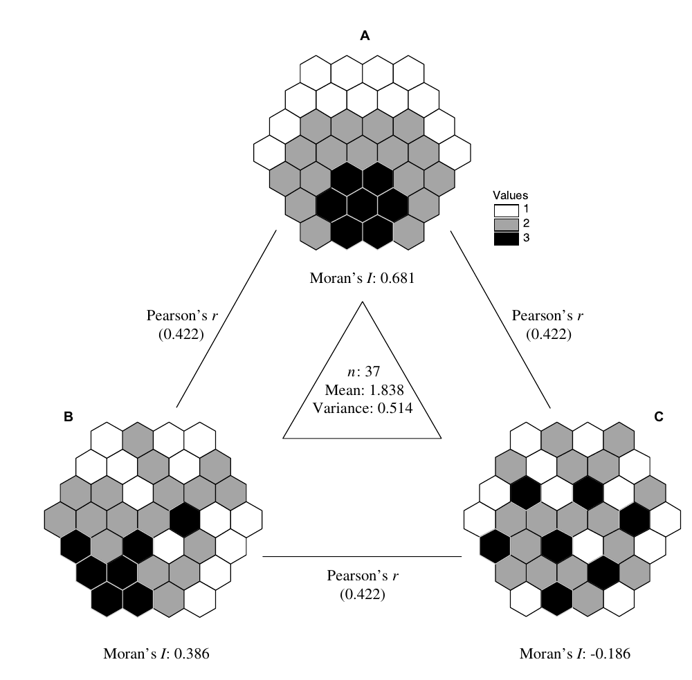
Figure 8.1: Correlation betwenn abservations A and B and C. B and C show identical values that are differently spatially arranged. Therefore, Pearson’s r is exaclty the same for A-B and A-C. However Moran’s I for B and C is different. As this effects the amount of information shared between neighboring observations, a measure that reflects that seems necessary.

Lee’s L measures bivariate spatial dependence, “a particular relationship between the spatial proximity among observational units and the numeric similarity of their bivariate associations”. If the distribution of bivariate associations is not spatially random, then bivariate spatial dependence exists.

We have already rewritten Moran’s I using the spatial lag operator above:

\[\tilde{x}_i = \sum_j w_{ij}x_j\]

\[ I = \frac{\sum_i^n (x_i - \bar{x}) (\tilde{x}_i - \bar{x}) } {\sqrt{\sum_i^n (x_i - \bar{x})^2 \sum_i^n (x_i - \bar{x})^2}}\]

If we now calculate Pearson’s r between the variable \(x\) and its lag \(\tilde{x}\) we can further rewrite the equation.

\[r_{x,\tilde{x}} = \frac{\sum_i(x_i-\bar{x})(\tilde{x}_i-\bar{x}))}{\sqrt{\sum_i(x_i-\bar{x})^2} \sqrt{\sum_i(x_i-\bar{x})^2}}\]

This allows us to write Moran’s I as:

\[I = \sqrt{\frac{\sum_i ( \tilde{x}_i -\bar{\tilde{x}})^2}{\sum_i ( x_i -\bar{x})^2}} \cdot r_{x,\tilde{x}}\]

This shows that Moran’s I is Pearson’s r between the variable and its spatial lag, scaled by the square root of the ratio of the variance of the spatial lagged variable and the variance of the variable.

If we rearrange the equation and use a clever approximation this can be further simplified (Lee, 2001).

\[I = \sqrt{\frac{\sum_i(\tilde{x}_i - \bar{x})^2}{\sum_i(\tilde{x}_i - \bar{x})^2}} \cdot \sqrt{\frac{\sum_i ( \tilde{x}_i -\bar{\tilde{x}})^2}{\sum_i ( x_i -\bar{x})^2}} \cdot r_{x,\tilde{x}} = \] \[ = \sqrt{\frac{\sum_i(\tilde{x}_i - \bar{x})^2}{\sum_i(x_i -\bar{x})^2}} \cdot \sqrt{\frac{\sum_i ( \tilde{x}_i -\bar{\tilde{x}})^2}{\sum_i ( \tilde{x}_i - \bar{x})^2}} \cdot r_{x,\tilde{x}} \]

As the mean of the original variable and its spatial lag can be expected to be very similar the can assume that \(\sqrt{\frac{\sum_i ( \tilde{x}_i -\bar{\tilde{x}})^2}{\sum_i ( \tilde{x}_i - \bar{x})^2}}\cong 1\).

\[I \cong \sqrt{\frac{\sum_i(\tilde{x}_i - \bar{x})^2}{\sum_i(x_i -\bar{x})^2}} 1 \cdot r_{x,\tilde{x}} = \sqrt{SSS} \cdot r_{x,\tilde{x}}\]

There \(SSS\) was termed spatial smoothing scalar by Lee (2001). If a variable is stronger spatially clustered, its SSS will be larger, as the variance of the original vector is less reduced when it is transformed to its spatial lag. SSS reveals substantive information about the spatial clustering of a variable. If a variable is stronger spatially clustered, its SSS is larger, because variance of the original vector is less reduced when it is transformed to its spatial lag.

SSS itself can be seen as a direction-free univariate spatial association measure that theoretically ranges from 0 to 1 (Lee, 2001).

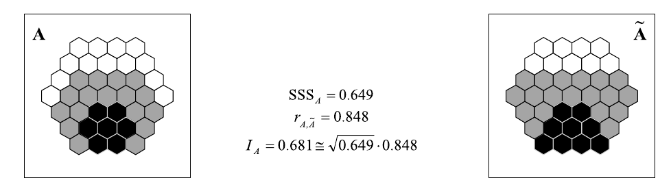
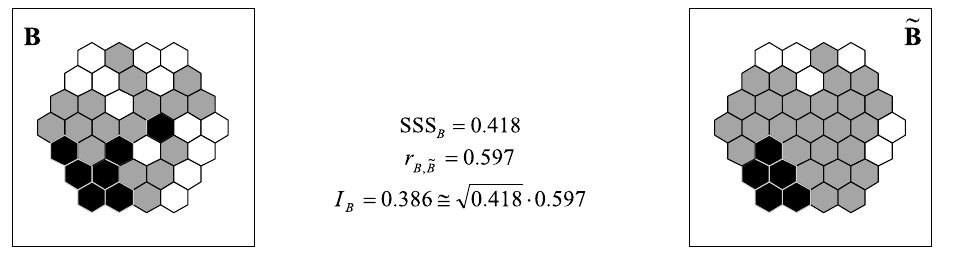
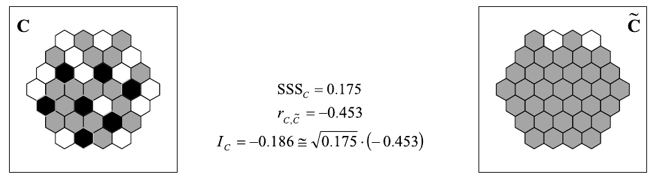
Lets have a look at three examples from Lee (2001). The figures show the spatial patternof the variable and of its spatial lag as well as the SSS, Pearson’s r for the variable and its spatial lag es well as Moran’s I.

For the bivariate case this can be extended to Lee’s L which can be rewritten as³:

\[L_{x,y}=\sqrt{SSS_y}\sqrt{SSS_y} \cdot r_{\tilde{x}, \tilde{y}} = \sqrt{BSSS_{x,y}} \cdot r_{\tilde{x}, \tilde{y}}\]

The equation can also be rearragned to:

\[L_{x,y} = \sqrt{L_{x,x}} \cdot \sqrt{L_{y,y}} \cdot r_{\tilde{x}, \tilde{y}}\]

We can also rearrange the bivariate Moran’s I formulas into:

\[I_{x,y} \cong \sqrt{SSS_y} \cdot r_{x, \tilde{y}}\]$

\[I_{y,x} \cong \sqrt{SSS_x} \cdot r_{y, \tilde{x}}\]

8.6 Simulated data

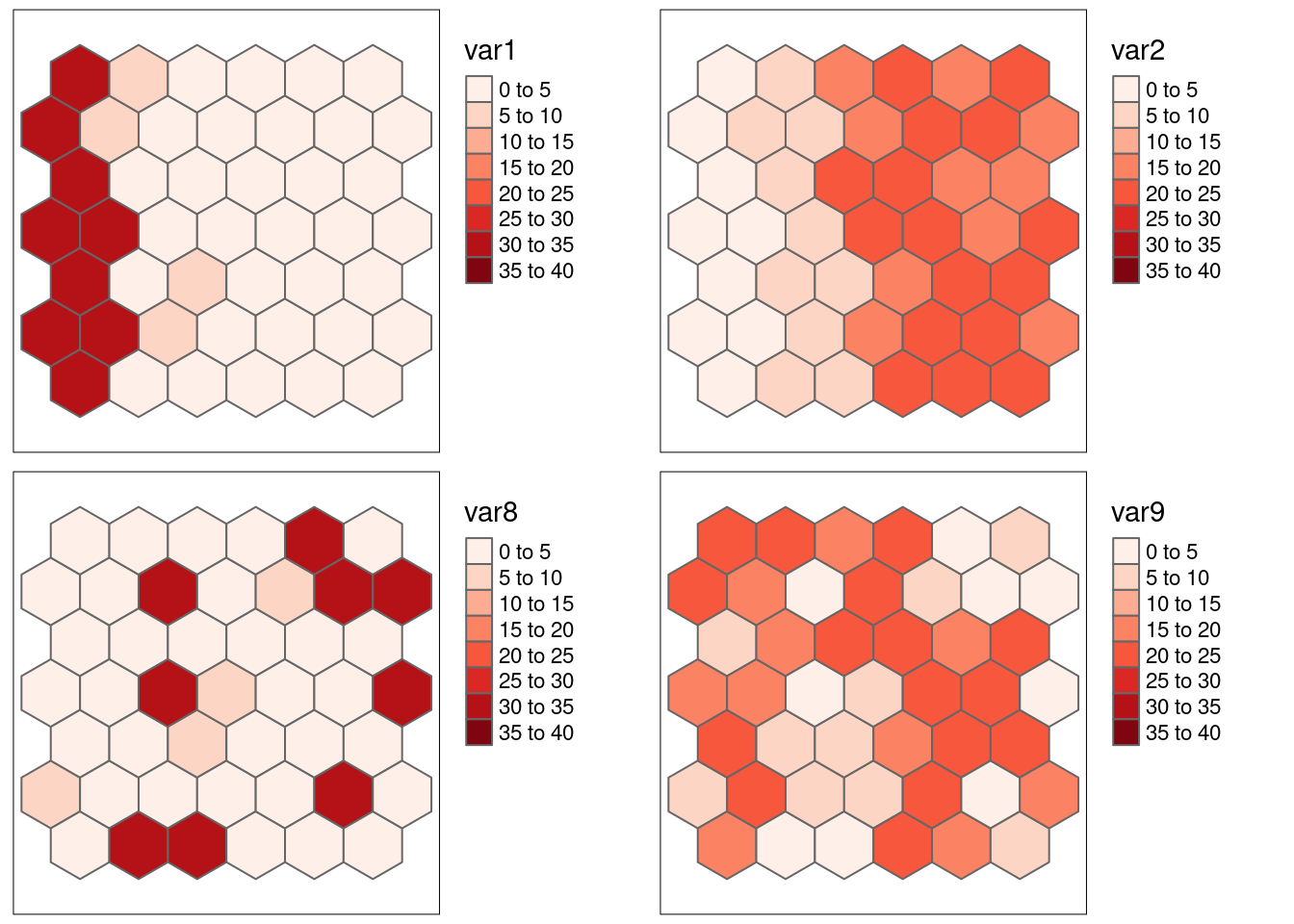
We create a hexagon tesselation and add some spatially structure columns to it that can then be used to explore Lee’s L for these pattern.

set.seed(3)
aoi <- st_sfc(st_polygon(list(rbind(c(0,0), c(5,0), c(5,5), c(0,0)))))
hexgrid <- st_make_grid(aoi,  cellsize = 1, square = FALSE)
hexgrid <- st_sf(hexgrid)

hexgrid <- st_sf(hexgrid, crs = 4326) # avoid warnings by assigning a CRS however, data is located nowhere


n <- nrow(hexgrid)
hexgrid$id <- 1:n

hexgrid <- hexgrid %>% mutate(var1 = ifelse(id <10, 30, ifelse(id < 20, 5, 1) + rnorm(n, mean= 0, sd=.1)),
                              var2 = ifelse(id <10, 2, ifelse(id < 20, 6, 20) + rnorm(n, mean= 0, sd=.1) ))

hexgrid <- hexgrid %>% mutate(var3 = rnorm(n, mean= 4) + var1,
                              var4 = rpois(n, lambda = var1),
                              var5 = rnorm(n, mean=30),
                              var6 = rnorm(n, mean=30))
hexgrid <- hexgrid %>% mutate(var7 = var6 + rnorm(n, mean= 0, sd=.5) )
idx <- sample(hexgrid$id, size=n, replace = FALSE)
hexgrid <- hexgrid %>% mutate(var8 = var1[idx], var9= var2[idx])
hexgrid <- hexgrid %>% mutate(var10 = var1 + rnorm(n))
hexgrid <- hexgrid %>% mutate(var11 = var10[idx])
hexgrid <- hexgrid %>% mutate(var1neg = max(var1)-1*var1)
hexgrid <- hexgrid %>% mutate(var12 = 10+ (id %%2) *10 - (id %%4)*2 - (id %%6)*2 + (id %% 8)*3)

hexgrid$var13 <- 20
hexgrid$var13[c(13, 14, 24, 35, 41, 30, 3, 5, 19, 40, 32, 18, 4)] <- 0
hexgrid$var13[c(23, 17,31, 37, 29, 15, 9, 17, 31, 43, 45 )] <- 40

hexgrid$var14 <- 0
hexgrid$var14[c(4:7, 18:21, 32:35)] <- 40
#tm_shape(hexgrid) + tm_polygons(col="var14") + tm_layout(legend.outside = TRUE) + tm_text(text="id")
# shift values of var1 one hexcell to the right (+ 7 ids)
# see tm_shape(hexgrid) + tm_polygons(col="id") + tm_layout(legend.outside = TRUE) + tm_text(text="id")
moveHex1toLeft <- function(id)
{ # only valid for this little hexgrid
  if(any(id>45)) {
    stop("id needs to be smaller than 45")
  }
    
  newid <- ifelse( (id >=4) & (id <= 7),
                  id +35,
                  ifelse(id < 4, 
                         id+42,
                         id-7))
  return(newid)
}

hexgrid <- hexgrid %>% mutate(var1shifted = var1[moveHex1toLeft(id)], 
                              var8shifted= var8[moveHex1toLeft(id)],
                              var13shifted= var13[moveHex1toLeft(id)],
                              var14shifted= var14[moveHex1toLeft(id)]
                              )

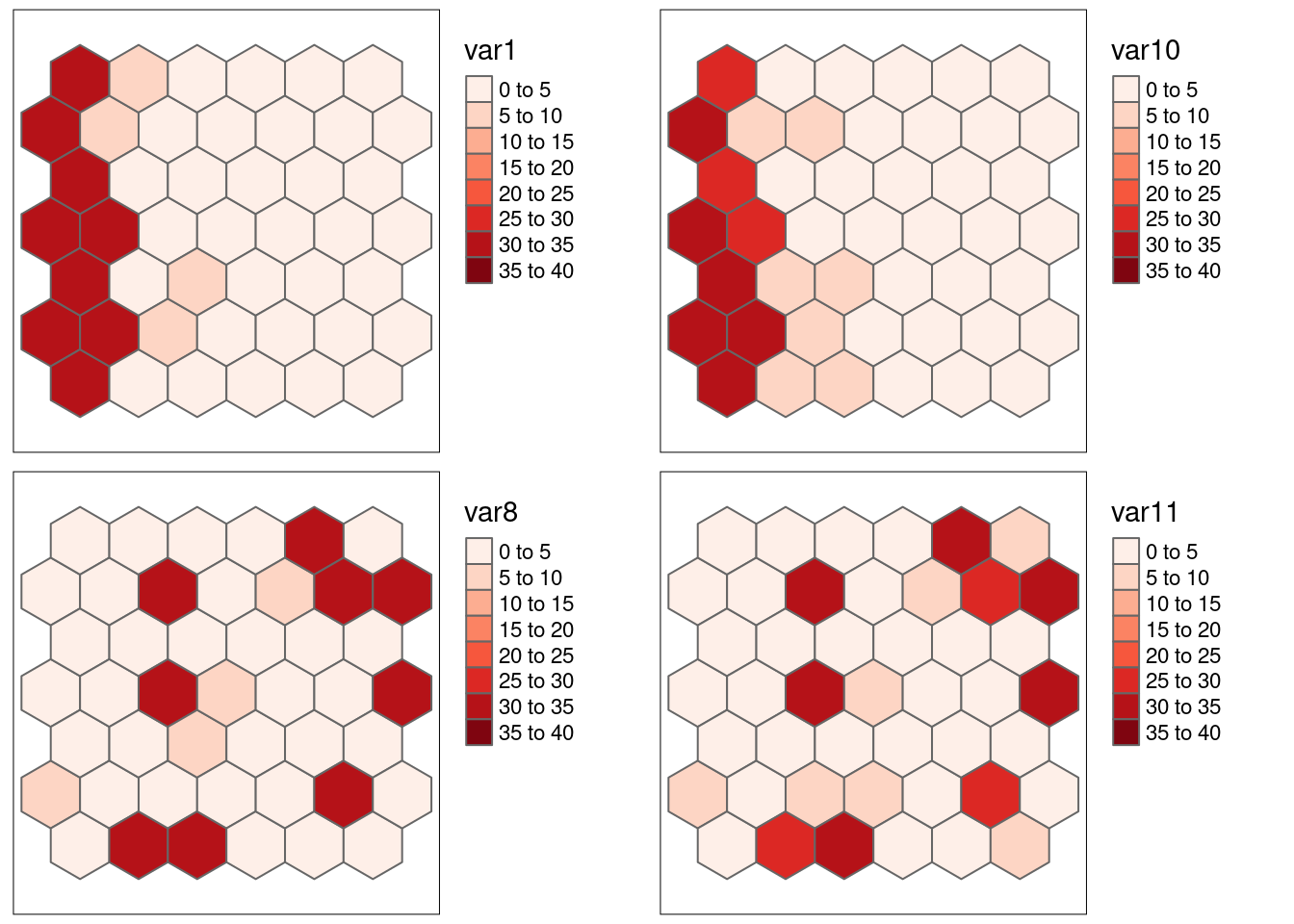
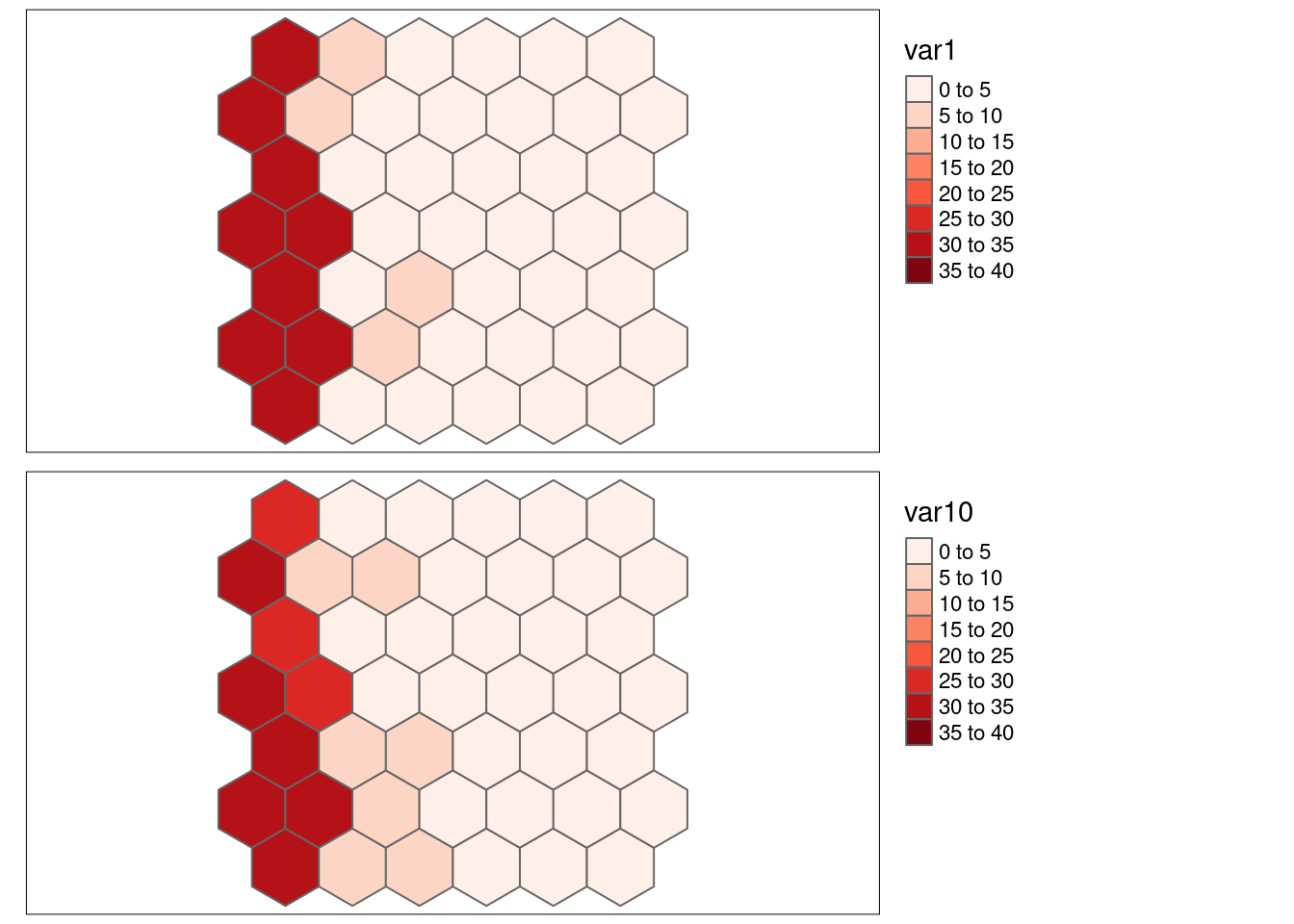
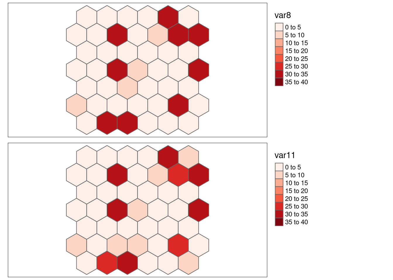
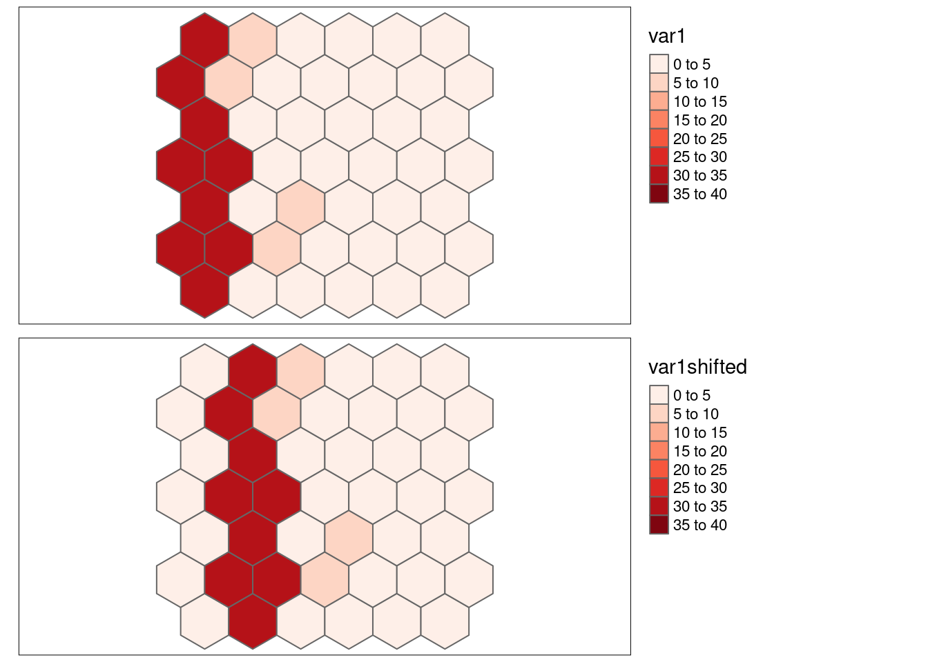
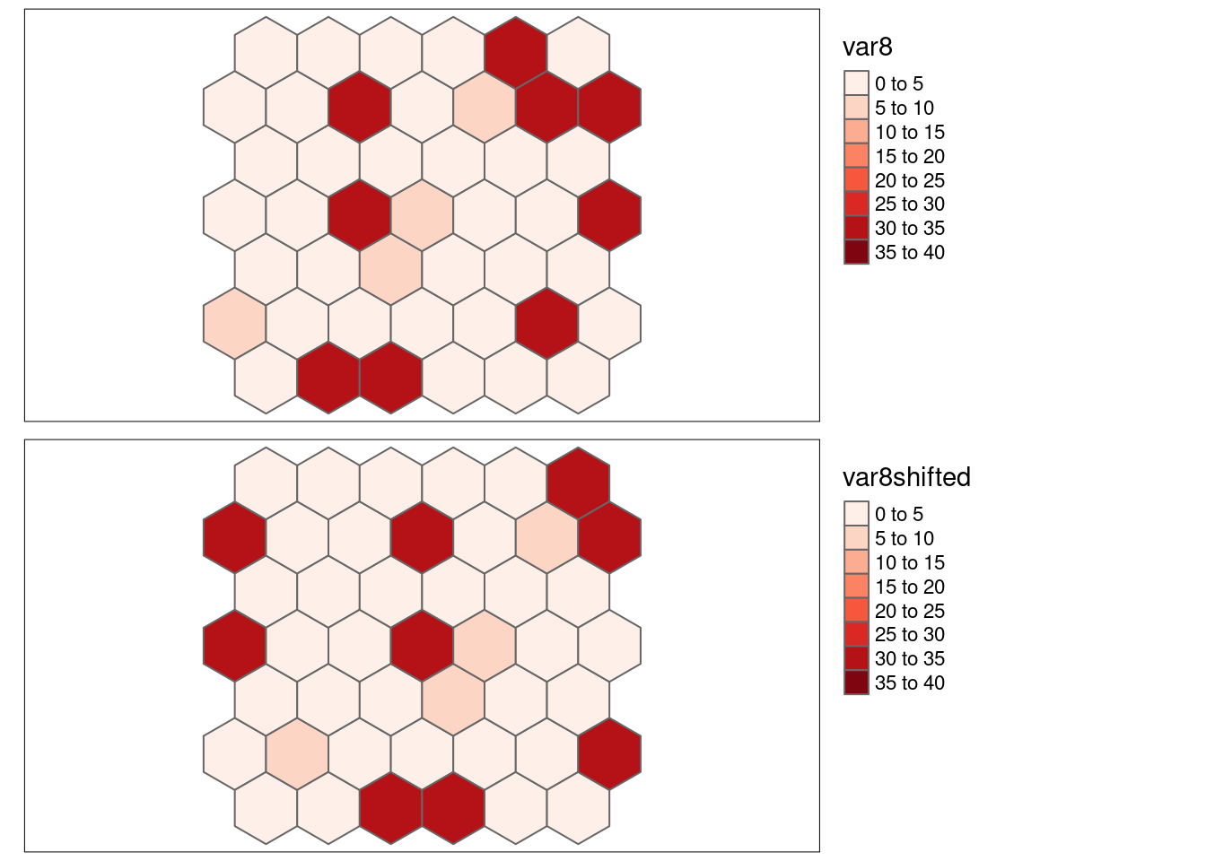
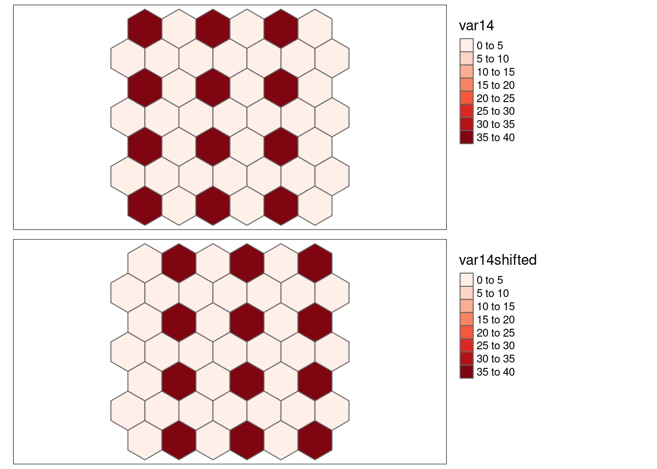
The simulated data (cf. 8.2) contains strongly positively correlated autocorrelation (e.g. var1 and var2), negative autocorrelation (e.g. var12 and var13) and random pattern (var1-6). For some we have simply reshuffled the locations of the data to break spatial structure (var1 and var2 have been reshuffled to var8 and var9) while for others the pattern has been simply shifted by one cell to the right (the varXshifted variables) or the patterns has been flipped (var1neg).

theBreaks <-seq(0,40, by=5)
thePalette <- "Reds"
m1 <- tm_shape(hexgrid) + tm_polygons(col="var1", breaks = theBreaks, palette= thePalette) +
  tm_layout(legend.outside = TRUE)
m2 <- tm_shape(hexgrid) + tm_polygons(col="var2", breaks = theBreaks, palette= thePalette) +
  tm_layout(legend.outside = TRUE)
m3 <- tm_shape(hexgrid) + tm_polygons(col="var3", breaks = theBreaks, palette= thePalette) +
  tm_layout(legend.outside = TRUE)
m4 <- tm_shape(hexgrid) + tm_polygons(col="var4", breaks = theBreaks, palette= thePalette) +
  tm_layout(legend.outside = TRUE)
m5 <- tm_shape(hexgrid) + tm_polygons(col="var5", breaks = theBreaks, palette= thePalette) +
  tm_layout(legend.outside = TRUE)
m6 <- tm_shape(hexgrid) + tm_polygons(col="var6", breaks = theBreaks, palette= thePalette) +
  tm_layout(legend.outside = TRUE)
m7 <- tm_shape(hexgrid) + tm_polygons(col="var7", breaks = theBreaks, palette= thePalette) +
  tm_layout(legend.outside = TRUE)
m8 <- tm_shape(hexgrid) + tm_polygons(col="var8", breaks = theBreaks, palette= thePalette) +
  tm_layout(legend.outside = TRUE)
m9 <- tm_shape(hexgrid) + tm_polygons(col="var9", breaks = theBreaks, palette= thePalette) +
  tm_layout(legend.outside = TRUE)
m10 <- tm_shape(hexgrid) + tm_polygons(col="var10", breaks = theBreaks, palette= thePalette) +
  tm_layout(legend.outside = TRUE)
m11 <- tm_shape(hexgrid) + tm_polygons(col="var11", breaks = theBreaks, palette= thePalette) +
  tm_layout(legend.outside = TRUE)
m12 <- tm_shape(hexgrid) + tm_polygons(col="var12", breaks = theBreaks, palette= thePalette) +
  tm_layout(legend.outside = TRUE)
m13 <- tm_shape(hexgrid) + tm_polygons(col="var13", breaks = theBreaks, palette= thePalette) +
  tm_layout(legend.outside = TRUE)
m14 <- tm_shape(hexgrid) + tm_polygons(col="var14", breaks = theBreaks, palette= thePalette) +
  tm_layout(legend.outside = TRUE)
m1neg <- tm_shape(hexgrid) + tm_polygons(col="var1neg", breaks = theBreaks, palette= thePalette) +
  tm_layout(legend.outside = TRUE)
m1shifted <- tm_shape(hexgrid) + tm_polygons(col="var1shifted", breaks = theBreaks, palette= thePalette) +
  tm_layout(legend.outside = TRUE)
m8shifted <- tm_shape(hexgrid) + tm_polygons(col="var8shifted", breaks = theBreaks, palette= thePalette) +
  tm_layout(legend.outside = TRUE)
m13shifted <- tm_shape(hexgrid) + tm_polygons(col="var13shifted", breaks = theBreaks, palette= thePalette) +
  tm_layout(legend.outside = TRUE)
m14shifted <- tm_shape(hexgrid) + tm_polygons(col="var14shifted", breaks = theBreaks, palette= thePalette) +
  tm_layout(legend.outside = TRUE)

tmap_arrange(m1,m2,m3,m4, m5, m6,m7, m8, m9, m10, m11, m12, m13, m14, m1neg, m1shifted, m8shifted, m13shifted, m14shifted)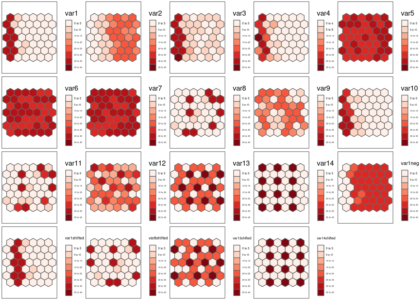

## Legend labels were too wide. The labels have been resized to 0.28, 0.23, 0.20, 0.20, 0.20, 0.20, 0.20, 0.20. Increase legend.width (argument of tm_layout) to make the legend wider and therefore the labels larger.
## Legend labels were too wide. The labels have been resized to 0.28, 0.23, 0.20, 0.20, 0.20, 0.20, 0.20, 0.20. Increase legend.width (argument of tm_layout) to make the legend wider and therefore the labels larger.
## Legend labels were too wide. The labels have been resized to 0.28, 0.23, 0.20, 0.20, 0.20, 0.20, 0.20, 0.20. Increase legend.width (argument of tm_layout) to make the legend wider and therefore the labels larger.

## Legend labels were too wide. The labels have been resized to 0.28, 0.28, 0.20, 0.20, 0.20, 0.20, 0.20, 0.20. Increase legend.width (argument of tm_layout) to make the legend wider and therefore the labels larger.

## Legend labels were too wide. The labels have been resized to 0.28, 0.23, 0.20, 0.20, 0.20, 0.20, 0.20, 0.20. Increase legend.width (argument of tm_layout) to make the legend wider and therefore the labels larger.
## Legend labels were too wide. The labels have been resized to 0.28, 0.23, 0.20, 0.20, 0.20, 0.20, 0.20, 0.20. Increase legend.width (argument of tm_layout) to make the legend wider and therefore the labels larger.
## Legend labels were too wide. The labels have been resized to 0.28, 0.23, 0.20, 0.20, 0.20, 0.20, 0.20, 0.20. Increase legend.width (argument of tm_layout) to make the legend wider and therefore the labels larger.
## Legend labels were too wide. The labels have been resized to 0.28, 0.23, 0.20, 0.20, 0.20, 0.20, 0.20, 0.20. Increase legend.width (argument of tm_layout) to make the legend wider and therefore the labels larger.
## Legend labels were too wide. The labels have been resized to 0.28, 0.23, 0.20, 0.20, 0.20, 0.20, 0.20, 0.20. Increase legend.width (argument of tm_layout) to make the legend wider and therefore the labels larger.
## Legend labels were too wide. The labels have been resized to 0.28, 0.23, 0.20, 0.20, 0.20, 0.20, 0.20, 0.20. Increase legend.width (argument of tm_layout) to make the legend wider and therefore the labels larger.
## Legend labels were too wide. The labels have been resized to 0.28, 0.23, 0.20, 0.20, 0.20, 0.20, 0.20, 0.20. Increase legend.width (argument of tm_layout) to make the legend wider and therefore the labels larger.
## Legend labels were too wide. The labels have been resized to 0.28, 0.23, 0.20, 0.20, 0.20, 0.20, 0.20, 0.20. Increase legend.width (argument of tm_layout) to make the legend wider and therefore the labels larger.
## Legend labels were too wide. The labels have been resized to 0.28, 0.23, 0.20, 0.20, 0.20, 0.20, 0.20, 0.20. Increase legend.width (argument of tm_layout) to make the legend wider and therefore the labels larger.
## Legend labels were too wide. The labels have been resized to 0.28, 0.23, 0.20, 0.20, 0.20, 0.20, 0.20, 0.20. Increase legend.width (argument of tm_layout) to make the legend wider and therefore the labels larger.
## Legend labels were too wide. The labels have been resized to 0.28, 0.23, 0.20, 0.20, 0.20, 0.20, 0.20, 0.20. Increase legend.width (argument of tm_layout) to make the legend wider and therefore the labels larger.
## Legend labels were too wide. The labels have been resized to 0.28, 0.23, 0.20, 0.20, 0.20, 0.20, 0.20, 0.20. Increase legend.width (argument of tm_layout) to make the legend wider and therefore the labels larger.
## Legend labels were too wide. The labels have been resized to 0.28, 0.23, 0.20, 0.20, 0.20, 0.20, 0.20, 0.20. Increase legend.width (argument of tm_layout) to make the legend wider and therefore the labels larger.
## Legend labels were too wide. The labels have been resized to 0.28, 0.23, 0.20, 0.20, 0.20, 0.20, 0.20, 0.20. Increase legend.width (argument of tm_layout) to make the legend wider and therefore the labels larger.
## Legend labels were too wide. The labels have been resized to 0.28, 0.23, 0.20, 0.20, 0.20, 0.20, 0.20, 0.20. Increase legend.width (argument of tm_layout) to make the legend wider and therefore the labels larger.

Figure 8.2: The following simulated patterns are analyzed later on with respect to Lee’s L.

A contiguity neighborhood definition is best suited for the case of the demonstration. This imples that each non-border cell has 6 neighbors while the border cells have less neighbors.

hexnb <- poly2nb(hexgrid)
hexlistw <- nb2listw(hexnb, style = "W")
hex_coord <- st_coordinates(hexgrid)[,1:2] # used later for the modified t-test

If we apply Moran’s test to the five simulated variables we see that all but the last three show significant spatial autocorrelation. (I am using sapply to map a function to a list but this is not of concern here.)

moran4vars <- lapply(2:8, FUN = function(x) moran.test(st_drop_geometry(hexgrid)[,x], listw = hexlistw))
moran4varsShorted <- sapply(moran4vars, FUN = function(x) c(x$estimate[1], x$p.value))
row.names(moran4varsShorted)[2] <- "p-value"
moran4varsShorted

##                           [,1]         [,2]         [,3]         [,4]
## Moran I statistic 6.778588e-01 8.140493e-01 6.773210e-01 6.101243e-01
## p-value           1.351183e-14 3.210743e-19 1.429188e-14 2.032328e-12
##                           [,5]       [,6]      [,7]
## Moran I statistic -0.007337836 0.01197456 0.1382407
## p-value            0.433931191 0.35233507 0.0370708

Let us explore the case of the obviously autocorrelated and shifted first two variables:

tmap_arrange(m1,m2)

lee.mc(hexgrid$var1, hexgrid$var2, listw = hexlistw, nsim = 499, alternative = "less")

## 
##  Monte-Carlo simulation of Lee's L
## 
## data:  hexgrid$var1 ,  hexgrid$var2 
## weights: hexlistw  
## number of simulations + 1: 500 
## 
## statistic = -0.63469, observed rank = 1, p-value = 0.002
## alternative hypothesis: less

cor.test(hexgrid$var1, hexgrid$var2)

## 
##  Pearson's product-moment correlation
## 
## data:  hexgrid$var1 and hexgrid$var2
## t = -8.7979, df = 43, p-value = 3.624e-11
## alternative hypothesis: true correlation is not equal to 0
## 95 percent confidence interval:
##  -0.8866491 -0.6646941
## sample estimates:
##        cor 
## -0.8017904

Compared to Pearson’s r that ignores spatial autocorrelation Lee’s L indicates a weaker but still clear negative association between var1 and var2.

Let’s repeat that with var3 which has added white noise.

tmap_arrange(m3,m2)

lee.mc(hexgrid$var3, hexgrid$var2, listw = hexlistw, nsim = 499, alternative = "less")

## 
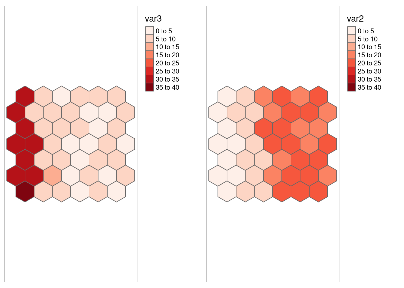
##  Monte-Carlo simulation of Lee's L
## 
## data:  hexgrid$var3 ,  hexgrid$var2 
## weights: hexlistw  
## number of simulations + 1: 500 
## 
## statistic = -0.6389, observed rank = 1, p-value = 0.002
## alternative hypothesis: less

cor.test(hexgrid$var3, hexgrid$var2)

## 
##  Pearson's product-moment correlation
## 
## data:  hexgrid$var3 and hexgrid$var2
## t = -8.828, df = 43, p-value = 3.294e-11
## alternative hypothesis: true correlation is not equal to 0
## 95 percent confidence interval:
##  -0.8872331 -0.6662194
## sample estimates:
##       cor 
## -0.802766

Similar. Both methods indicate significant negative correlation between var2 and var3. Lee’s L is against smaller due to the effect of positive spatial autocorrelation in the data.

For the two white noise variables without spatial structure both association measures indicate expectedly no significant relationship.

tmap_arrange(m5,m6)

lee.mc(hexgrid$var6, hexgrid$var5, listw = hexlistw, nsim = 499, alternative = "less")

## 
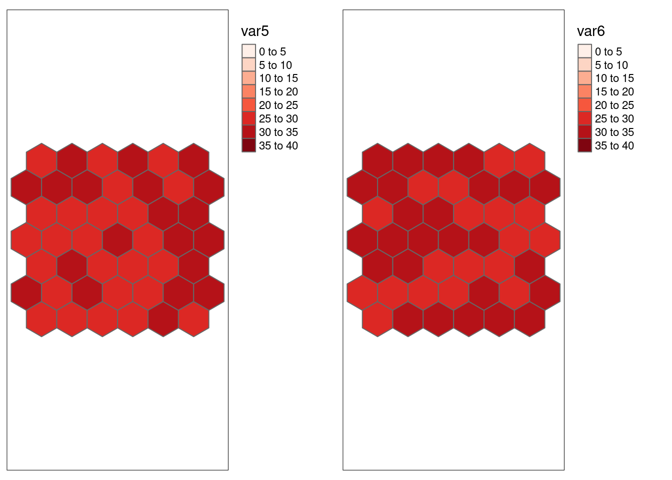
##  Monte-Carlo simulation of Lee's L
## 
## data:  hexgrid$var6 ,  hexgrid$var5 
## weights: hexlistw  
## number of simulations + 1: 500 
## 
## statistic = 0.061969, observed rank = 425, p-value = 0.85
## alternative hypothesis: less

cor.test(hexgrid$var6, hexgrid$var5)

## 
##  Pearson's product-moment correlation
## 
## data:  hexgrid$var6 and hexgrid$var5
## t = 0.79209, df = 43, p-value = 0.4327
## alternative hypothesis: true correlation is not equal to 0
## 95 percent confidence interval:
##  -0.179947  0.399396
## sample estimates:
##       cor 
## 0.1199212

The last case is interesting as we are comparing two variables without significant spatial autocorrelation that were designed to be correlated. While Pearson’s r indicates strong autocorrelation, Lee’´s L suggest no significant association.

tmap_arrange(m7,m6)

lee.mc(hexgrid$var6, hexgrid$var7, listw = hexlistw, nsim = 999, alternative = "greater")

## 
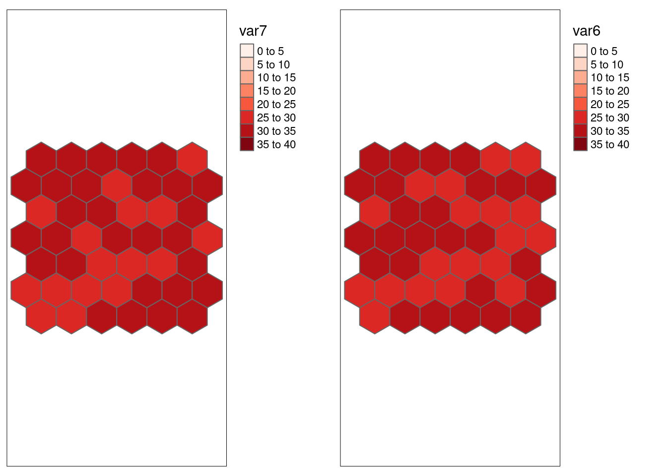
##  Monte-Carlo simulation of Lee's L
## 
## data:  hexgrid$var6 ,  hexgrid$var7 
## weights: hexlistw  
## number of simulations + 1: 1000 
## 
## statistic = 0.169, observed rank = 574, p-value = 0.426
## alternative hypothesis: greater

cor.test(hexgrid$var6, hexgrid$var7)

## 
##  Pearson's product-moment correlation
## 
## data:  hexgrid$var6 and hexgrid$var7
## t = 8.9585, df = 43, p-value = 2.178e-11
## alternative hypothesis: true correlation is not equal to 0
## 95 percent confidence interval:
##  0.6727348 0.8897199
## sample estimates:
##       cor 
## 0.8069249

8.6.1 Examples

We are looking here at a number of cases in a bit more detail. The idea is to present simple cases that make it easier to spot and understand differences in the metrics calculated for the pattern. Of course, real world cases will be more complicated - if you think of those as a mixture of such archetypes of relationships it might help you to understand the meaning of Lee’s L.

This section is still a stub with very limited explanation. This should hopefully change in the not so far future.

8.6.1.1 Helper functions

To ease the code we define some functions for the calculation of the different indicators.

# functions for calculating spatial smoothing scalar
calcSSS <- function(values, listw, zero.policy=NULL)
{
  # calc spatial lag
  values.lag <- lag.listw(x=listw, var=values, zero.policy = zero.policy )
  values.mean <- mean(values)
  sssx <- sum((values.lag-values.mean)^2) / sum((values-values.mean)^2)
  return(sssx)
}

calcPearsonLagged <- function(x,y, listw, zero.policy=NULL)
{
  xlag<- lag.listw(x=listw, var=x, zero.policy = zero.policy )
  ylag<- lag.listw(x=listw, var=y, zero.policy = zero.policy )
  res <- cor(xlag, ylag)
  return(res)
}

calcSpatialCorrIndicators <- function(var1, var2, listw, 
                          zero.policy=NULL, nsim = 499, 
                          alternative = "greater", scale = TRUE)
{
  if(length(var1) != length(var2))
    stop("calcSpatialCorrIndicators: var1 and var2 differ in length")
  # if(length(var1) != length(hexlistw$neighbours))
  #   stop("calcSpatialCorrIndicators: length listw does not fit var1 and var2") 
  if(!(alternative %in% c("greater", "less", "two.sided")))
    stop("calcSpatialCorrIndicators: alternative needs to be one of 'greater', 'less', 'two.side'")
  
  # SSS for var 1
  sssVar1 <- calcSSS(var1, listw = listw, zero.policy= zero.policy)
  # SSS for var 2
  sssVar2 <- calcSSS(var2, listw = listw, zero.policy= zero.policy)
  # pearson's r for lagged var1 and lagged var2
  rXlayLag <- calcPearsonLagged(var1, var2, listw = listw)
  # Moran's I for var1
  Ix <- moran.test(var1, listw = listw, 
                   zero.policy= zero.policy, 
                   alternative= alternative)$estimate[1] %>% as.numeric()
  # Moran's I for var2
  Iy <- moran.test(var2, listw = listw, 
                   zero.policy= zero.policy, 
                   alternative= alternative)$estimate[1] %>% as.numeric()
  # Lee's L
  leeVar1Var2 <- lee.mc(var1, var2, listw = listw, 
                   zero.policy= zero.policy, 
                        nsim = nsim,
                        alternative= alternative)$statistic %>% as.numeric()
  # pearson's r for var1 and var2
  rXY <- cor(var1, var2)
  # bivariate Moran's I
  bv_1_2 <- moran_bv(var1, var2, listw = listw,  
                     nsim = nsim, scale = scale)$t0
  bv_2_1 <- moran_bv(var2, var1, listw = listw, 
                     nsim = nsim, scale = scale)$t0
  
  res <- list(sssVar1 = sssVar1,
              sssVar2 = sssVar2,
              rXlayLag = rXlayLag,
              Ix = Ix, Iy = Iy,
              leeVar1Var2 = leeVar1Var2,
              rXY = rXY,
              bv_1_2 = bv_1_2,
              bv_2_1 = bv_2_1)
  return(res)
}

printSpatialCorrIndicators <- function(indi, n.signif=3)
{
  cat(paste("r =\t", indi$rXY %>% signif(n.signif)), "\n")
  cat(paste("r_lx,ly =", indi$rXlayLag %>% signif(n.signif)), "\n")
  
  cat(paste("SSS_x =\t", indi$sssVar1 %>% signif(n.signif)), "\n" )
  cat(paste("SSS_y =\t", indi$sssVar2 %>% signif(n.signif)), "\n")
  
  cat(paste("L_x,y =\t", indi$leeVar1Var2 %>% signif(n.signif)), "\n")
  
  cat(paste("I_x =\t", indi$Ix %>% signif(n.signif)), "\n")
  cat(paste("I_y =\t", indi$Iy %>% signif(n.signif)), "\n")
  
  cat(paste("I_B(x,y) =", indi$bv_1_2 %>% signif(n.signif)), "\n")
  cat(paste("I_B(y,x) =", indi$bv_2_1 %>% signif(n.signif)), "\n")
}

8.6.1.2 Strong positive autocorrelation, same values

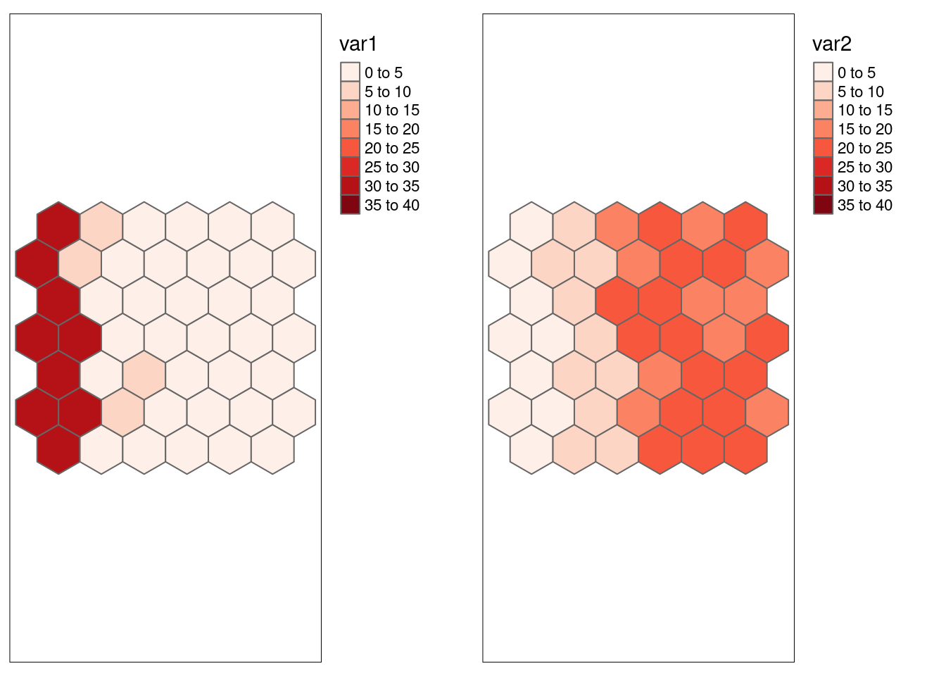
Here we are looking at the bivariate association of var1with itself.

indi <- calcSpatialCorrIndicators(hexgrid$var1, hexgrid$var1, listw = hexlistw)

tmap_arrange(m1,m1, nrow = 2)

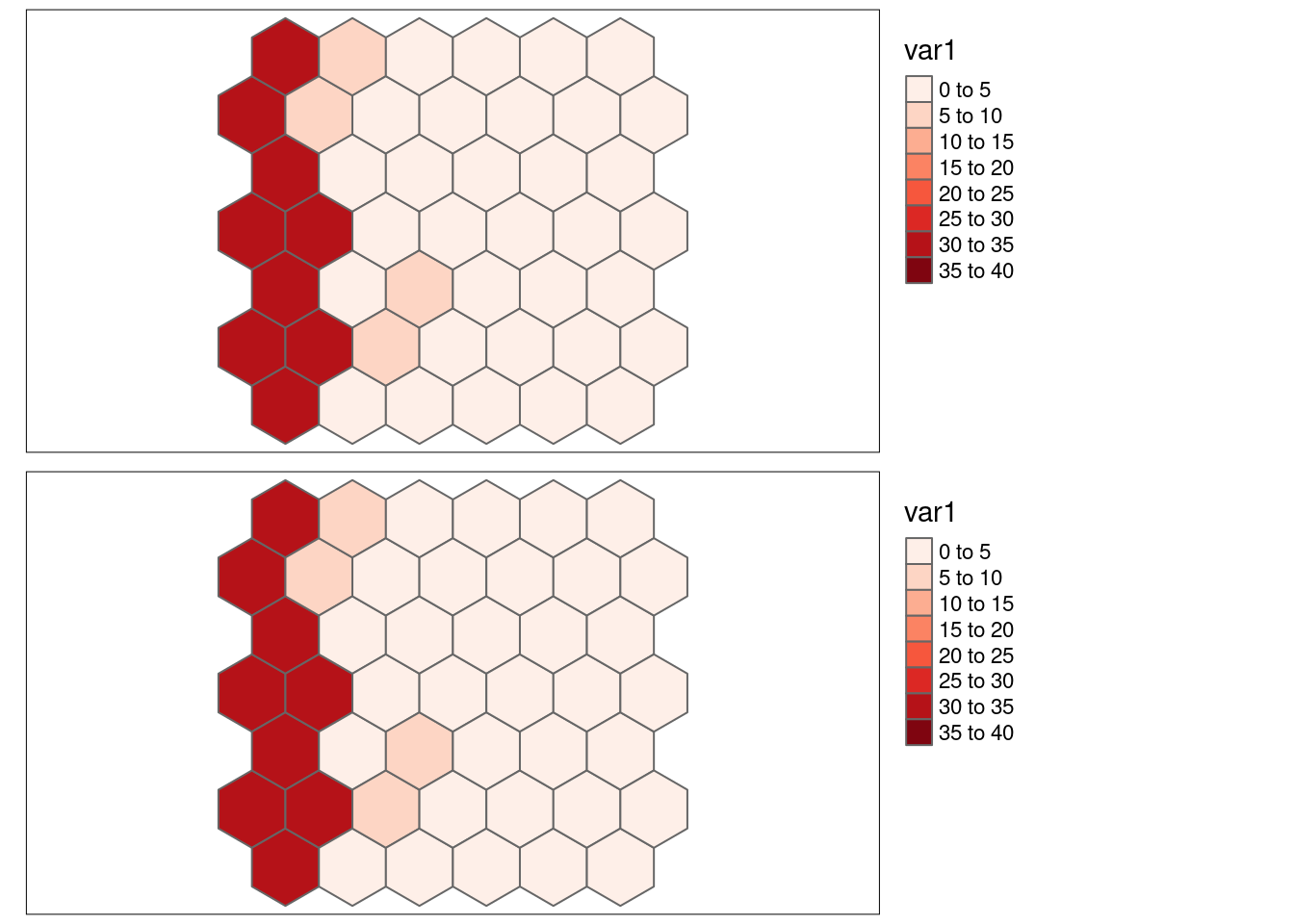
• \(SSS_{x}\) = 0.6112571
• \(SSS_{y}\) = 0.6112571
• \(r_{\tilde{x}, \tilde{y}}\) = 1
• \(L_{x,y}\) = 0.6112571
• \(I_x\) = 0.6778588
• \(I_y\) = 0.6778588
• r = 1
• \(L_{x,y}=\sqrt{SSS_x}\sqrt{SSS_y} \cdot r_{\tilde{x}, \tilde{y}}\)
• \(I_{B}(x,y)\) = 0.6778588

8.6.1.3 Strong positive autocorrelation, inverse values

var1neg has been created such that it shows a strong positive autocorrelation but the vaues are kind of inverted with respect to var1, leading to a negative Pearson’s r.

indi <- calcSpatialCorrIndicators(hexgrid$var1, hexgrid$var1neg, listw = hexlistw)

tmap_arrange(m1, m1neg, nrow = 2)

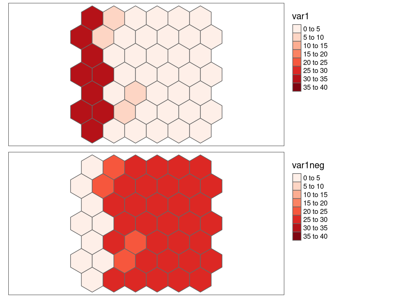
• \(SSS_{x}\) = 0.6112571
• \(SSS_{y}\) = 0.6112571
• \(r_{\tilde{x}, \tilde{y}}\) = -1
• \(L_{x,y}\) = -0.6112571
• \(I_x\) = 0.6778588
• \(I_y\) = 0.6778588
• r = -1
• \(I_{B}(x,y)\) = -0.6778588

8.6.1.4 Negative autocorrelation, same values

Here we look at the different measures for the bivariate association of an example with (weak) negative spatial autocorrelation var12 with it self.

indi <- calcSpatialCorrIndicators(hexgrid$var12, hexgrid$var12, listw = hexlistw)

tmap_arrange(m12, m12, nrow = 2)

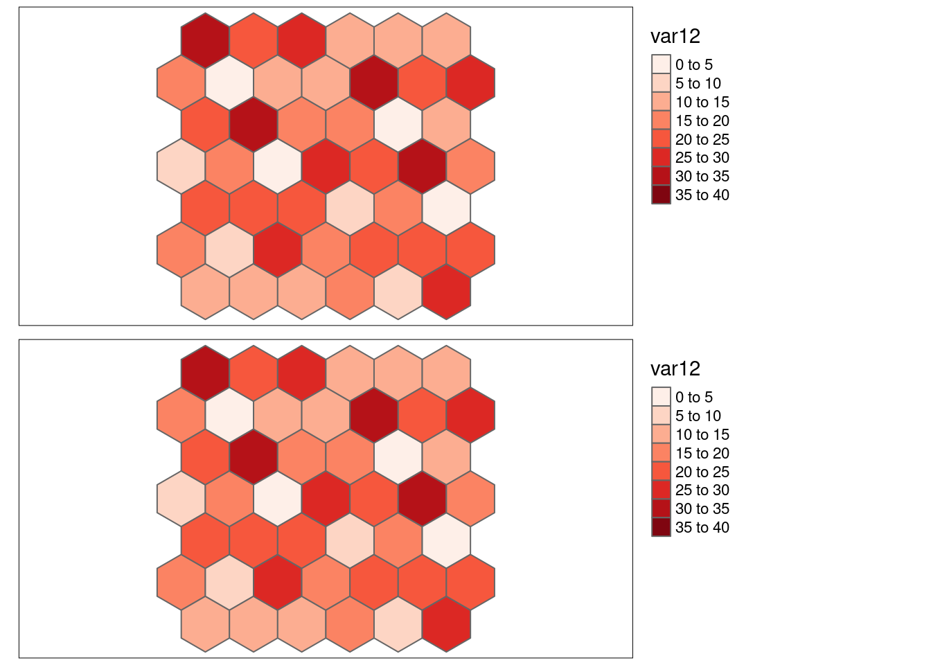
• \(SSS_{x}\) = 0.1340738
• \(SSS_{y}\) = 0.1340738
• \(r_{\tilde{x}, \tilde{y}}\) = 1
• \(L_{x,y}\) = 0.1340738
• \(I_x\) = -0.3083754
• \(I_y\) = -0.3083754
• r = 1
• \(I_{B}(x,y)\) = -0.3083754

8.6.1.5 Strong positive autocorrelation, contrary pattern

var2has been created such that it has a strong positive spatial autocorrelation but that high values of var2 are linked to low values for var1, leading to a negative association.

indi <- calcSpatialCorrIndicators(hexgrid$var1, hexgrid$var2, listw = hexlistw)

tmap_arrange(m1,m2, nrow = 2)

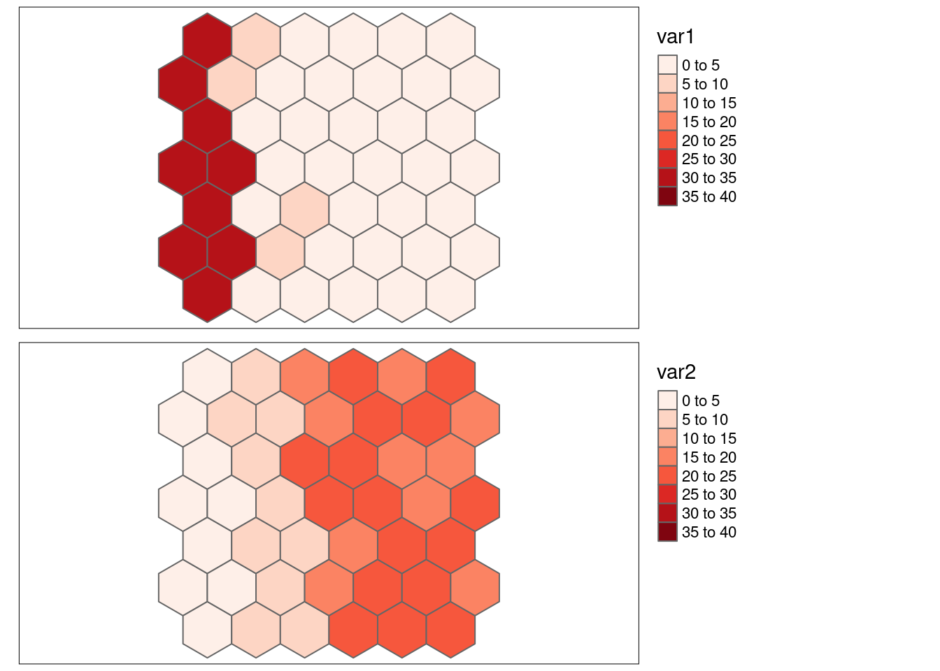
• \(SSS_{x}\) = 0.6112571
• \(SSS_{y}\) = 0.7654227
• \(r_{\tilde{x}, \tilde{y}}\) = -0.9281803
• \(L_{x,y}\) = -0.6346862
• \(I_x\) = 0.6778588
• \(I_y\) = 0.8140493
• r = -0.8017904
• \(I_{B}(x,y)\) = -0.6976358
• \(I_{B}(y,x)\) = -0.6725747

8.6.1.6 Example: var1 and var2, rearranged

Now we look at shuffled versions of var1 and var2: both variables were rearranged in exactly the same way, i.e. the observations still correspond. However, Moran’s I has changed as the shuffeling broke the spatial autocorrelation. var8 corresponds to the values in var1 and var9 to the values in var2.

The scatterplots look exactly the same:

p1 <- ggplot(hexgrid, aes(x=var1, y= var2)) +
  geom_point() + labs(title = "Original")
p2 <- ggplot(hexgrid, aes(x=var8, y= var9)) +
  geom_point()  + labs(title = "Reshuffled")
ggarrange(p1,p2)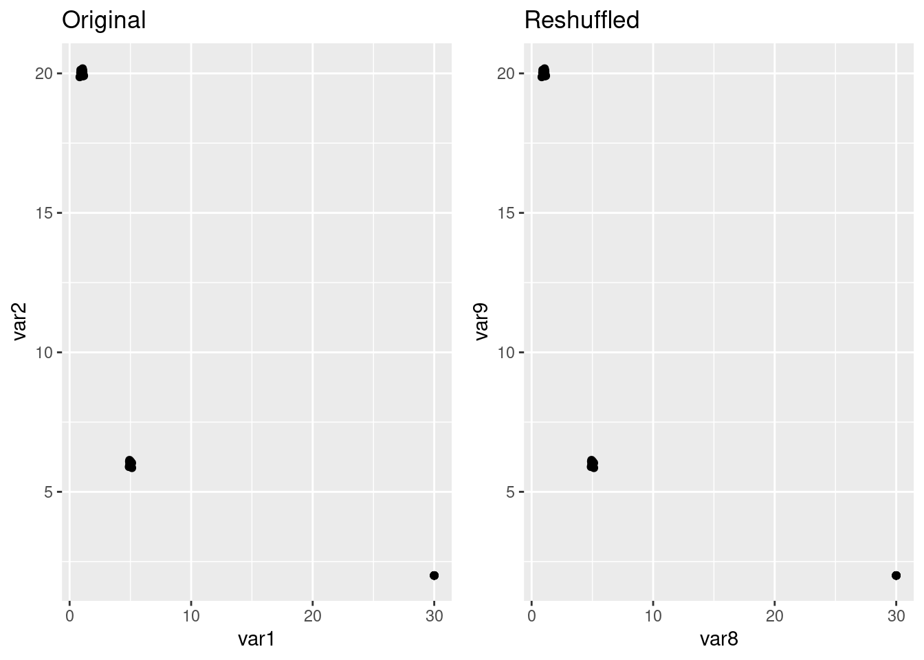

tmap_arrange(m1,m2, m8, m9)

Let’s have a look at Moran’s I

varPos <- c(1,2,8,9)
moran4vars <- lapply(varPos+1, FUN = function(x) moran.test(st_drop_geometry(hexgrid)[,x], listw = hexlistw))
moran4varsShorted <- sapply(moran4vars, FUN = function(x) c(x$estimate[1], x$p.value))
row.names(moran4varsShorted)[2] <- "p-value"
colnames(moran4varsShorted) <- paste0("var", varPos)
t(moran4varsShorted)

##      Moran I statistic      p-value
## var1        0.67785884 1.351183e-14
## var2        0.81404932 3.210743e-19
## var8       -0.03219664 5.409725e-01
## var9        0.05562954 2.027172e-01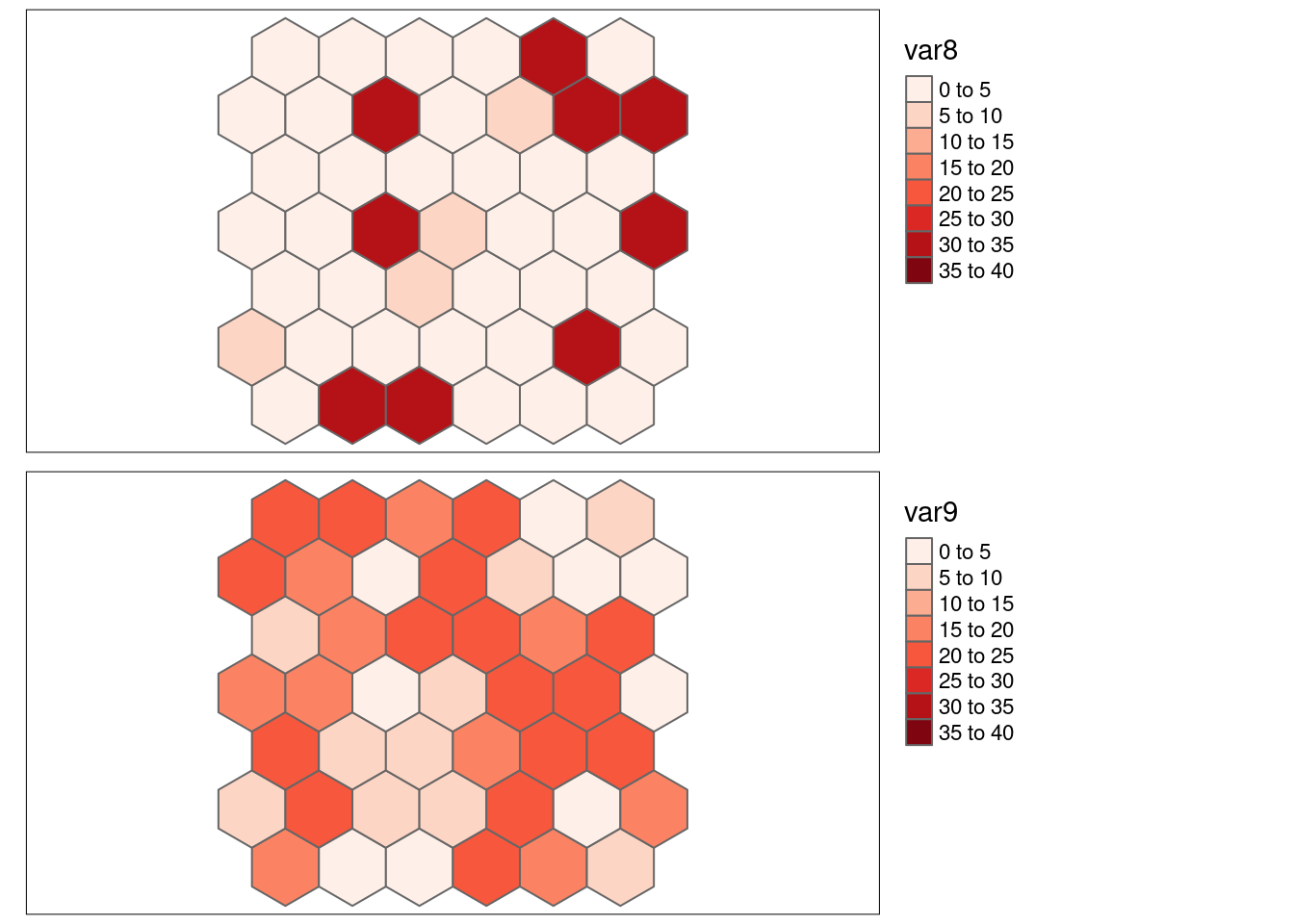

indi <- calcSpatialCorrIndicators(hexgrid$var8, hexgrid$var9, listw = hexlistw)

tmap_arrange(m8,m9, nrow = 2)

::: ::: {.column} - \(SSS_{x}\) = 0.221982 - \(SSS_{y}\) = 0.2366627 - \(r_{\tilde{x}, \tilde{y}}\) = -0.8358157 - \(L_{x,y}\) = -0.1915687 - \(I_x\) = -0.0321966 - \(I_y\) = 0.0556295 - r = -0.8017904 - \(I_{B}(x,y)\) = -0.0200969 - \(I_{B}(y,x)\) = -0.0259268

Lee’s L for var8 and var9 shows no significant spatial pattern of bivariate association.

lee.mc(hexgrid$var8, hexgrid$var9, listw = hexlistw, nsim = 499, alternative = "less")

## 
##  Monte-Carlo simulation of Lee's L
## 
## data:  hexgrid$var8 ,  hexgrid$var9 
## weights: hexlistw  
## number of simulations + 1: 500 
## 
## statistic = -0.19157, observed rank = 114, p-value = 0.228
## alternative hypothesis: less

Lee’s L for var1 and var2 shows a clear negative bivariate spatial association. The positive spatial autocorrelation present in var1 and var2 increased Lee’ L.

lee.mc(hexgrid$var1, hexgrid$var2, listw = hexlistw, nsim = 499, alternative = "less")

## 
##  Monte-Carlo simulation of Lee's L
## 
## data:  hexgrid$var1 ,  hexgrid$var2 
## weights: hexlistw  
## number of simulations + 1: 500 
## 
## statistic = -0.63469, observed rank = 1, p-value = 0.002
## alternative hypothesis: less

Pearson’s r did not change (by definition) between var1and var2and for var8and var9.

cor.test(hexgrid$var8, hexgrid$var9)

## 
##  Pearson's product-moment correlation
## 
## data:  hexgrid$var8 and hexgrid$var9
## t = -8.7979, df = 43, p-value = 3.624e-11
## alternative hypothesis: true correlation is not equal to 0
## 95 percent confidence interval:
##  -0.8866491 -0.6646941
## sample estimates:
##        cor 
## -0.8017904

The significance of the test for Pearson’s r is not really changed if the look at the modified t-test

var1 vs. var2

modified.ttest(hexgrid$var1, hexgrid$var2, coords= hex_coord)

## 
## Corrected Pearson's correlation for spatial autocorrelation
## 
## data: x and y ; coordinates: X and Y 
## F-statistic: 51.8097 on 1 and 28.7818 DF, p-value: 0 
## alternative hypothesis: true autocorrelation is not equal to 0
## sample correlation: -0.8018

var8 vs. var9

modified.ttest(hexgrid$var8, hexgrid$var9, coords= hex_coord)

## 
## Corrected Pearson's correlation for spatial autocorrelation
## 
## data: x and y ; coordinates: X and Y 
## F-statistic: 43.7545 on 1 and 24.3069 DF, p-value: 0 
## alternative hypothesis: true autocorrelation is not equal to 0
## sample correlation: -0.8018

8.6.1.7 Positive correlation with and without positive spatial autocorrelation var1-var10 and var8-var11 (reshuffled)

tmap_arrange(m1,m10, m8, m11)

Scatterplot

p1 <- ggplot(hexgrid, aes(x=var1, y= var10)) +
  geom_point() + labs(title = "Original")
p2 <- ggplot(hexgrid, aes(x=var8, y= var11)) +
  geom_point()  + labs(title = "Reshuffled")
ggarrange(p1,p2)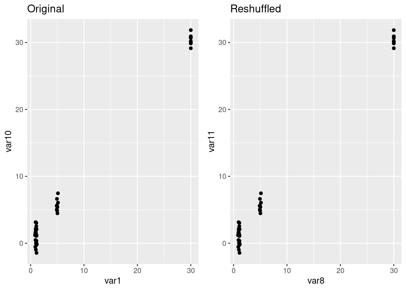

Pearson’s r var1 vs. var10

cor.test(hexgrid$var1, hexgrid$var10)

## 
##  Pearson's product-moment correlation
## 
## data:  hexgrid$var1 and hexgrid$var10
## t = 71.789, df = 43, p-value < 2.2e-16
## alternative hypothesis: true correlation is not equal to 0
## 95 percent confidence interval:
##  0.9924220 0.9977336
## sample estimates:
##       cor 
## 0.9958542

Pearson’s r var8 vs. var11

cor.test(hexgrid$var8, hexgrid$var11)

## 
##  Pearson's product-moment correlation
## 
## data:  hexgrid$var8 and hexgrid$var11
## t = 71.789, df = 43, p-value < 2.2e-16
## alternative hypothesis: true correlation is not equal to 0
## 95 percent confidence interval:
##  0.9924220 0.9977336
## sample estimates:
##       cor 
## 0.9958542

Lee’s L var1 vs. var10

lee.mc(hexgrid$var1, hexgrid$var10, listw = hexlistw, nsim = 499, alternative = "two.sided")

## 
##  Monte-Carlo simulation of Lee's L
## 
## data:  hexgrid$var1 ,  hexgrid$var10 
## weights: hexlistw  
## number of simulations + 1: 500 
## 
## statistic = 0.61188, observed rank = 500, p-value < 2.2e-16
## alternative hypothesis: two.sided

• spatial rearrangement makes the pattern less similar according to Lee’s L
• as the positive spatial autocorrelation in var1 and var10 is destroyed thereby
• Pearson’s r cannot capture that as it does not consider the spatial pattern

Lee’s L var8 vs. var11

lee.mc(hexgrid$var8, hexgrid$var11, listw = hexlistw, nsim = 499, alternative = "two.sided")

## 
##  Monte-Carlo simulation of Lee's L
## 
## data:  hexgrid$var8 ,  hexgrid$var11 
## weights: hexlistw  
## number of simulations + 1: 500 
## 
## statistic = 0.21908, observed rank = 344, p-value = 0.624
## alternative hypothesis: two.sided

Moran’s I var1-var10 & var8-var11

varPos <- c(1,10,8,11)
moran4vars <- lapply(varPos+1, FUN = function(x) moran.test(st_drop_geometry(hexgrid)[,x], listw = hexlistw))
moran4varsShorted <- sapply(moran4vars, FUN = function(x) c(x$estimate[1], x$p.value))
row.names(moran4varsShorted)[2] <- "p-value"
colnames(moran4varsShorted) <- paste0("var", varPos)
t(moran4varsShorted)

##       Moran I statistic      p-value
## var1         0.67785884 1.351183e-14
## var10        0.68308295 9.003126e-15
## var8        -0.03219664 5.409725e-01
## var11       -0.03448282 5.507866e-01

8.6.1.7.1 Strong positive autocorrelation, positive association

indi <- calcSpatialCorrIndicators(hexgrid$var1, hexgrid$var10, listw = hexlistw)

tmap_arrange(m1,m10, nrow = 2)

• \(SSS_{x}\) = 0.6112571
• \(SSS_{y}\) = 0.613609
• \(r_{\tilde{x}, \tilde{y}}\) = 0.9990976
• \(L_{x,y}\) = 0.6118786
• \(I_x\) = 0.6778588
• \(I_y\) = 0.6830829
• r = 0.9958542
• \(I_{B}(x,y)\) = 0.6794298
• \(I_{B}(y,x)\) = 0.6820743

8.6.1.7.2 Strong positive autocorrelation, positive association

indi <- calcSpatialCorrIndicators(hexgrid$var8, hexgrid$var11, listw = hexlistw)

tmap_arrange(m8,m11, nrow = 2)

• \(SSS_{x}\) = 0.221982
• \(SSS_{y}\) = 0.2180351
• \(r_{\tilde{x}, \tilde{y}}\) = 0.9958227
• \(L_{x,y}\) = 0.2190766
• \(I_x\) = -0.0321966
• \(I_y\) = -0.0344828
• r = 0.9958542
• \(I_{B}(x,y)\) = -0.0332237
• \(I_{B}(y,x)\) = -0.0339476

8.6.1.8 Strong positive autocorrelation, shifted by one cell

indi <- calcSpatialCorrIndicators(hexgrid$var1, hexgrid$var1shifted, listw = hexlistw)

tmap_arrange(m1,m1shifted, nrow = 2)

• \(SSS_{x}\) = 0.6112571
• \(SSS_{y}\) = 0.4151456
• \(r_{\tilde{x}, \tilde{y}}\) = 0.6660567
• \(L_{x,y}\) = 0.3317141
• \(I_x\) = 0.6778588
• \(I_y\) = 0.3445732
• r = 0.0919851
• \(I_{B}(x,y)\) = 0.3812871
• \(I_{B}(y,x)\) = 0.2708408

8.6.1.9 No autocorrelation, shifted by one cell

indi <- calcSpatialCorrIndicators(hexgrid$var8, hexgrid$var8shifted, listw = hexlistw)

tmap_arrange(m8,m8shifted, nrow = 2)

• \(SSS_{x}\) = 0.221982
• \(SSS_{y}\) = 0.1194423
• \(r_{\tilde{x}, \tilde{y}}\) = 0.2263546
• \(L_{x,y}\) = 0.0355491
• \(I_x\) = -0.0321966
• \(I_y\) = -0.0383465
• r = 0.0094375
• \(I_{B}(x,y)\) = 0.0742934
• \(I_{B}(y,x)\) = 0.1074713

8.6.1.10 Negative autocorrelation, shifted by one cell

indi <- calcSpatialCorrIndicators(hexgrid$var14, hexgrid$var14shifted, listw = hexlistw)

tmap_arrange(m14,m14shifted, nrow = 2)

• \(SSS_{x}\) = 0.2121212
• \(SSS_{y}\) = 0.2121212
• \(r_{\tilde{x}, \tilde{y}}\) = -0.6571019
• \(L_{x,y}\) = -0.1378788
• \(I_x\) = -0.3454545
• \(I_y\) = -0.3454545
• r = -0.3636364
• \(I_{B}(x,y)\) = 0.1545455
• \(I_{B}(y,x)\) = 0.1545455

8.7 The COVID-19 data case study - bivariate association

We will use the covid-19 incidence data for Germany that have been introduced previously.

covidKreise <- st_read(dsn = "data/covidKreise.gpkg", layer = "kreiseWithCovidMeldeWeeklyCleaned")

## Reading layer `kreiseWithCovidMeldeWeeklyCleaned' from data source 
##   `/home/slautenbach/Documents/lehre/HD/git_areas/spatial_data_science/spatial-data-science/data/covidKreise.gpkg' 
##   using driver `GPKG'
## Simple feature collection with 400 features and 145 fields
## Geometry type: MULTIPOLYGON
## Dimension:     XY
## Bounding box:  xmin: 280371.1 ymin: 5235856 xmax: 921292.4 ymax: 6101444
## Projected CRS: ETRS89 / UTM zone 32N

polynb <- poly2nb(covidKreise)
poSurfKreise <- st_point_on_surface(covidKreise)

## Warning: st_point_on_surface assumes attributes are constant over geometries

distnb <- dnearneigh(poSurfKreise, d1=1, d2= 70*10^3)
unionedNb <- union.nb(distnb, polynb)
dlist <- nbdists(unionedNb, st_coordinates(poSurfKreise))
dlist <- lapply(dlist, function(x) 1/x)
unionedListw_d <- nb2listw(unionedNb, glist=dlist, style = "W")
ebiMc <- EBImoran.mc(n= st_drop_geometry(covidKreise)%>% pull("sumCasesTotal"),
              x= covidKreise$EWZ, listw = unionedListw_d, nsim =999)

## The default for subtract_mean_in_numerator set TRUE from February 2016

8.7.1 Incidence vs. votes for right winged party

Let’s look at the association between the transformed response variable (empirical bayes modification) with two variables we will be using later on as predictors in our model: the votes for the right winged party at the national election in 2017 (Stimmenanteile.AfD) and the rurality of a district (Laendlichkeitmeasured as the share of population that lives in densely populated areas in the district).

First the normal Pearson correlation coefficient:

cor.test(x = covidKreise$Stimmenanteile.AfD, y = ebiMc$z)

## 
##  Pearson's product-moment correlation
## 
## data:  covidKreise$Stimmenanteile.AfD and ebiMc$z
## t = 10.226, df = 398, p-value < 2.2e-16
## alternative hypothesis: true correlation is not equal to 0
## 95 percent confidence interval:
##  0.3748636 0.5304747
## sample estimates:
##       cor 
## 0.4561491

cor.test(x = covidKreise$Laendlichkeit, y = ebiMc$z)

## 
##  Pearson's product-moment correlation
## 
## data:  covidKreise$Laendlichkeit and ebiMc$z
## t = 3.6908, df = 398, p-value = 0.0002547
## alternative hypothesis: true correlation is not equal to 0
## 95 percent confidence interval:
##  0.08538521 0.27505941
## sample estimates:
##       cor 
## 0.1819139

When Lee’s L with the permutation test:

lee.mc(x = covidKreise$Stimmenanteile.AfD, y = ebiMc$z, 
       listw = unionedListw_d, nsim = 999)

## 
##  Monte-Carlo simulation of Lee's L
## 
## data:  covidKreise$Stimmenanteile.AfD ,  ebiMc$z 
## weights: unionedListw_d  
## number of simulations + 1: 1000 
## 
## statistic = 0.35156, observed rank = 1000, p-value = 0.001
## alternative hypothesis: greater

lee.mc(x = covidKreise$Laendlichkeit, y = ebiMc$z, 
       listw = unionedListw_d, nsim = 999)

## 
##  Monte-Carlo simulation of Lee's L
## 
## data:  covidKreise$Laendlichkeit ,  ebiMc$z 
## weights: unionedListw_d  
## number of simulations + 1: 1000 
## 
## statistic = 0.11064, observed rank = 1000, p-value = 0.001
## alternative hypothesis: greater

We see that the incorporation of spatial autocorrelation reduces the estimated strength of the relationship as both variables are positively spatially autocorrelated. As the spatial autocorrelation for rurality is weaker this leads to a lower difference bettwen Pearson’s r and Lee’s L.

moran.mc(covidKreise$Stimmenanteile.AfD, listw= unionedListw_d, nsim = 999)

## 
##  Monte-Carlo simulation of Moran I
## 
## data:  covidKreise$Stimmenanteile.AfD 
## weights: unionedListw_d  
## number of simulations + 1: 1000 
## 
## statistic = 0.73757, observed rank = 1000, p-value = 0.001
## alternative hypothesis: greater

moran.mc(covidKreise$Laendlichkeit, listw= unionedListw_d, nsim = 999)

## 
##  Monte-Carlo simulation of Moran I
## 
## data:  covidKreise$Laendlichkeit 
## weights: unionedListw_d  
## number of simulations + 1: 1000 
## 
## statistic = 0.22267, observed rank = 1000, p-value = 0.001
## alternative hypothesis: greater

In summary:

• both variables (weakly) positively correlated

• spatial lag of both variables also (weakly) positively correlated

• both variables strong positive global spatial autocorrelation

• positive bivariate spatial dependence (similarity)

• r = -0.364

• \(r_{\tilde{x}, \tilde{y}}\) = -0.657

• \(I_x\) = -0.345

• \(I_y\) = -0.345

• \(SSS_{x}\) = 0.212

• \(SSS_{y}\) = 0.212

• \(L_{x,y}\) = -0.138

• \(I_{B}(x,y)\) = 0.155

• \(I_{B}(y,x)\) = 0.155

8.7.2 Fast internet availibility and rurality

covm1 <- tm_shape(covidKreise) + tm_polygons(col="Breitbandversorgung",
                         legend.reverse = TRUE, title = "Fast internet") +
  tm_layout(legend.outside = TRUE, bg.color = "darkgrey", outer.bg.color = "lightgrey",
            legend.outside.size = 0.5, attr.outside = TRUE,
            legend.outside.position = "left") + tm_scale_bar()

covm2 <- tm_shape(covidKreise) + tm_polygons(col="Laendlichkeit",  palette= "-plasma",
                         legend.reverse = TRUE, title = "Rurality") +
  tm_layout(legend.outside = TRUE, bg.color = "darkgrey", outer.bg.color = "lightgrey",
            legend.outside.size = 0.5, attr.outside = TRUE, 
            legend.outside.position = "right") + tm_scale_bar()

tmap_arrange(covm1, covm2)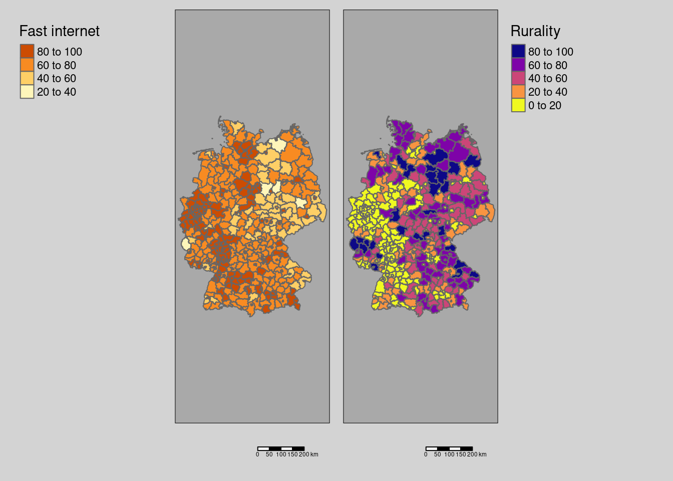

indi <- calcSpatialCorrIndicators(covidKreise$Breitbandversorgung, covidKreise$Laendlichkeit, listw = unionedListw_d)

• both variables negatively correlated

• spatial lag of both variables also negatively correlated

• both variables weak positive global spatial autocorrelation

• negative bivariate spatial dependence (disimilarity)

• \(r_{x,y}\) = -0.741

• \(r_{\tilde{x}, \tilde{y}}\) = -0.783

• \(I_x\) = 0.233

• \(I_y\) = 0.223

• \(SSS_{x}\) = 0.303

• \(SSS_{y}\) = 0.267

• \(L_{x,y}\) = -0.223

• \(I_{B}(x,y)\) = -0.168

• \(I_{B}(y,x)\) = -0.166

8.7.3 Share of students and share foreigners

covm1 <- tm_shape(covidKreise) + tm_polygons(col="Studierende", style="jenks",
                         legend.reverse = TRUE, title = "Students by 1000 inh.") +
  tm_layout(legend.outside = TRUE, bg.color = "darkgrey", outer.bg.color = "lightgrey",
            legend.outside.size = 0.5, attr.outside = TRUE, 
            legend.outside.position = "left") + tm_scale_bar()

covm2 <- tm_shape(covidKreise) + tm_polygons(col="Auslaenderanteil",  palette= "-plasma",
                         legend.reverse = TRUE, title = "Share foreigners") +
  tm_layout(legend.outside = TRUE, bg.color = "darkgrey", outer.bg.color = "lightgrey",
            legend.outside.size = 0.5, attr.outside = TRUE, 
            legend.outside.position = "right") + tm_scale_bar()

tmap_arrange(covm1, covm2)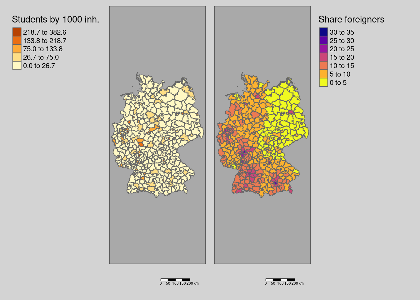

indi <- calcSpatialCorrIndicators(covidKreise$Studierende, covidKreise$Auslaenderanteil, listw = unionedListw_d)

• both variables (weakly) positively correlated

• spatial lag of both variables also (weakly) positively correlated

• share of foreigners positive global spatial autocorrelation

• no bivariate spatial dependence

• \(r_{x,y}\) = 0.381

• \(r_{\tilde{x}, \tilde{y}}\) = 0.374

• \(I_x\) = -0.0626

• \(I_y\) = 0.467

• \(SSS_{x}\) = 0.0546

• \(SSS_{y}\) = 0.488

• \(L_{x,y}\) = 0.0616

• \(I_{B}(x,y)\) = 0.0104

• \(I_{B}(y,x)\) = 0.0112

References

Clifford, P., Richardson, S., Hemon, D., 1989. Assessing the Significance of the Correlation between Two Spatial Processes. Biometrics 45, 123. https://doi.org/10.2307/2532039

Dutilleul, P., Clifford, P., Richardson, S., Hemon, D., 1993. Modifying the t Test for Assessing the Correlation Between Two Spatial Processes. Biometrics 49, 305. https://doi.org/10.2307/2532625

Lee, S.-I., 2001. Developing a bivariate spatial association measure: An integration of Pearson’s r and Moran’s I. Journal of Geographical Systems 3, 369–385. https://doi.org/10.1007/s101090100064

---

3. see Lee (2001) for details↩︎