Chapter 14 Geostatistics - kriging
require(raster)
library(terra)
require(sf)
require(sp)
require(tmap)
require(gstat)
require(tidyverse)
14.1 Cheat sheet
We use the gstat package for the geostatistic analysis. Important commands are:
gstat::variogram- deriving an empirical semi-variogramgstat::variogram.fit- fitting a theoretical semi-variogramgstat::vgm- defining a semi-variogram modelgstat::krige- performing the interpolationgstat::fitlmcFit a Linear Model of Coregionalization to a Multivariable Sample Variogram- organizing variables (and models) for cokriging
gstat::gstat - crosvalidation
gstat::krige.cvorgstat::gstat.cv
14.2 tl;dr - Geostatistics, kriging and interpolation in a nutshell
Geostatistics is concerned with the analysis of spatial processes based on a sample of observations. A common application is interpolation, i.e. an estimation of the underlying spatial process. We will also concentrate on this application here. However, geostatistics covers a much wider domain.
Similar to simpler interpolation approaches such as IDW or natural neighbor interpolation kriging can be used to estimates response values at locations without measurements. Similar to the simpler interpolation approaches, kriging uses both the measurements of the response and the location of the measurements. The estimated value at a location without measurements is calculated as the weighted sum of the measurements. The (kriging) weights add up to 1 and are calculated based on a function of the distance of the location to be interpolated and the sample locations. The calculation is based on a function (theoretical semi-variogram) which has been fitted to the data (empirical semi-variogram). This is the main difference to approaches such as IDW - the kriging weights results from fitting a model. This allows also an estimation of the uncertainty of the prediction of response values at locations without measurements.
Kriging relies on assumptions about spatial stationary. This implies that it is necessary to remove the effect of covariates or of spatial trends beforehand.
Kriging based interpolation in R using the gstat package consists at the core of the following steps:
- deriving an empirical semi-variogram using
variogram - fitting a theoretical semi-variogram using
variogram.fit - performing the interpolation using
krigeorprediction
14.3 Kriging - theory
We assume a real-valued, spatially continuous stochastic process \(S(X)\) that represents the real world phenomena we are interested in, e.g. the long term average air temperature at 2m above ground or the copper concentration in the topsoil. The process is unknown but we have observations/measurements \(Y_i\) at sample locations \(x_i\). We might impose additional constraints on \(S(X)\), e.g. that it is continuous or (many-times) differentiable. We might as well allow discrepancies between the true surface \(S(X)\) and measurements \(Y_i\), e.g. due to measurement errors.
The simplest model for that purpose is a stationary Gaussian model. It is defined as follows (Diggle and Ribeiro, 2007):
- {\(S(x): x \epsilon R^2\)} is a Gaussian process with mean \(\mu = E[S(x)]\), variance \(\sigma^2\) and correlation function \(\rho(u) = Corr(S(x), S(x'))\) where \(u\) is the distance between \(x\) and \(x'\) (\(||x-x'||\)). || || is the euclidian distance.
- \(y_i\) are realizations of mutually independent random variables \(Y_i\), normally distributed with conditional means \(E[Y_i|S(.)]=S(x_i)\) and conditional variances \(\tau^2\)
An equivalent formulation is:
\[Y_i = S(x_i) + Z_i, i=1,...n\]
where \(Z_i\) are mutually independent random variable from a normal distribution with zero mean and \(\tau^2\) variance.
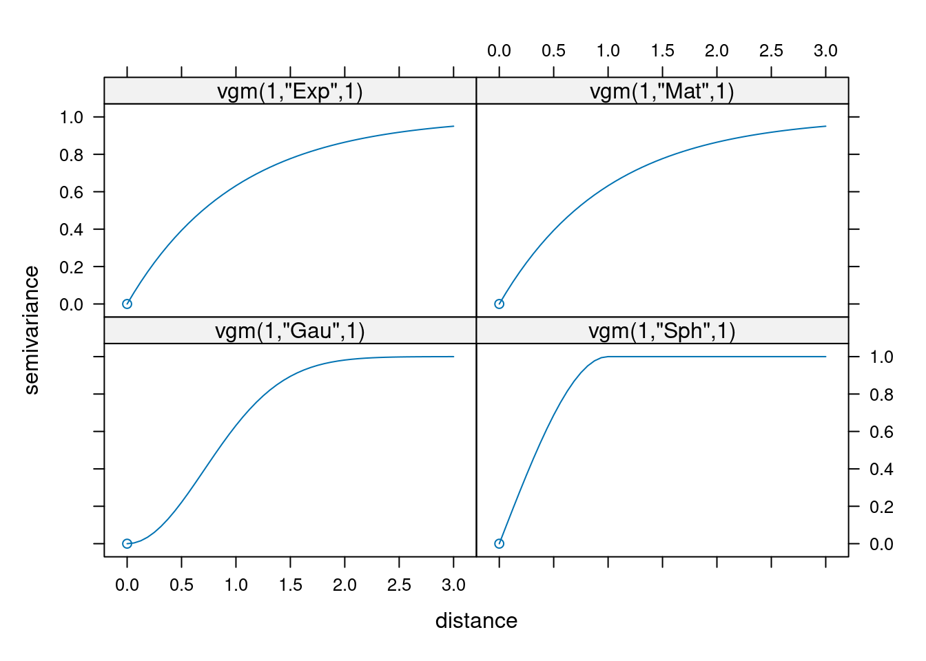
The correlation function \(\rho(u)\) needs to be positive definite for a legitimate model - in simple words the variance needs to be positive. This imposes non-obvious constraints. In practice this means that a few standard classes are used for \(\rho(u)\). These standard classes involve the Matérn, Gaussian, Exponential and the Spherical model.
Estimation of \(S(X)\) is based on modelling the covariance between observations, based on the semi-variogram, which is related to the correlation function.
14.3.1 Stationarity
For many operations in the context of kriging we assume a stationary process.
A spatial Gaussian process is stationary if:
- \(\mu(x) = \mu\) for all \(x\), i.e. the mean function is constant and does not depend on the location or covariates, and
- \(\gamma(x,x') = \gamma(u)\), where \(u= x-x'\), i.e. the covariance between \(S(x)\) at two locations depends only on the vector difference between \(x\) and \(x'\)
A stationary process is isotropic if \(\gamma(u) = \gamma(||u||)\), i.e. the covariance between \(S(x)\) at two locations depends only on the distance between them (and not on the direction).
The variance of a stationary process is constant: \(\sigma^2 = \gamma(0)\).
The correlation function is defined as \(\rho(u) = \frac{\gamma(u)}{\sigma^2}\). The correlation function is symmetric: \(\rho(u) = \rho(-u)\).
Estimating \(S(X)\) for a stationary gaussian process is called ordinary kriging.
If the mean function depends on covariates and location (spatial trend), we can still apply kriging, if \(S(x)-\mu(x)\) is stationary (covariance stationary). In other words: for some processes we can reach stationarity if we correct for the effect of the location and of covariates. This is what is widely used in practice - this is called universal kriging.
14.3.2 Variogram
The variogram of a spatial stochastic process \(S(x)\) is the following function:
\[ V(x,x') = \frac{1}{2} Var(S(x)-S(x')) = \frac{1}{2} (Var(S(x)) + Var(S(x')) - 2 Cov(S(x), S(x')) )\]
which simplifies to \(V(u) = \sigma^2(1-\rho(u))\) for stationary processes. Due to the factor 1/2 the variogram is also called semi-variogram. It is theoretically equivalent to the covariance function but has advantages, especially if the data locations originate from a irregular spatial design.
The semi-variance is also commonly expressed as a function of the distance band between observations:
\[ \gamma(h) = \frac{1}{2}E[(z(s_i) - z(s_i+h))^2] \] where \(z(s_i)\) is the value of the target variable (e.g. temperature) at some sample location \(i\) and \(z(s_i+h)\) the value of the target variable of the neighbor at distance \(h\). Frequently, we do not look at individual distance pairs but at the semi-variance averaged across a specific distance band (or lag).
14.3.3 Correlation functions
Typically, for stationary covariance structures the correlation between \(S(x)\) and \(S(x')\) decreases as the distance \(u= ||x-x'||\) increases. Therefore, correlation functions frequently show such behavior.
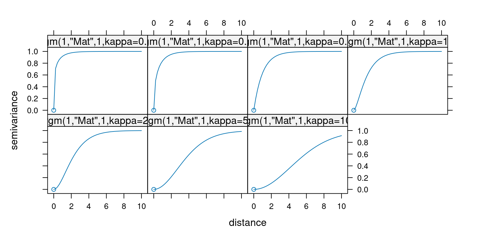
The Matérn family of correlation functions describes such a decrease in correlation (increase in the variogram) with increasing distances between two locations \(S(x)\) and \(S(x')\). It is defined as follows:
\[ \rho(u) = \frac{1}{2^{\kappa-1} \Gamma(\kappa)}(\frac{u}{\phi})^{\kappa} K_{\kappa} (\frac{u}{\phi})\] where \(K_{\kappa}\) denotes a modified Bessel function of order \(\kappa\), \(\phi > 0\) is a scale parameter with the dimensions of distance and \(\kappa\) > 0, the order is a shape parameter that determines the smoothness of the underlying process \(S(x)\).
For \(\kappa=0.5\) the Matérn correlation function reduces to the exponential correlation function: \(\rho(u) = e^{-\frac{u}{\phi}}\).
For \(kappa \to \infty\) the Matérn correlation function reduces to the Gaussian correlation function: \(\rho(u) = e^{-(\frac{u}{\phi})^2}\).
The spherical correlation function is defined as follows:
\[ \rho(u) = \begin{cases} 1 - \frac{3}{2} \frac{u}{\phi} + \frac{1}{2}(\frac{u}{\phi})^3 & : 0 \geq u \geq \phi \\ 0 & : u > \phi \end{cases} \]
Based on the different correlation functions (which describe a functional form), we can fit a theoretical variogram to the semi-variogram, derived from the data. We pick a function (such as the spherical correlation function and the corresponding functional relationship for the semi-variogram) and specify the parameters that provide the best fit for the data. The fitting is based on a weighted non-linear least square approach for gaussian processes. The weights used are often defined as \(N_j/h_j^2\), there \(N_j\) is the number of distance pairs in the j-th bin and \(h_j\) is the distance. This implies that the fitting process puts more weight on bins with more distance pairs and at shorter distance.
14.3.4 Variogram plots
The variograms for these four functions look as follows:
The following plots show the effect of different values for \(\kappa\) on the shape of the Matern family variogram.
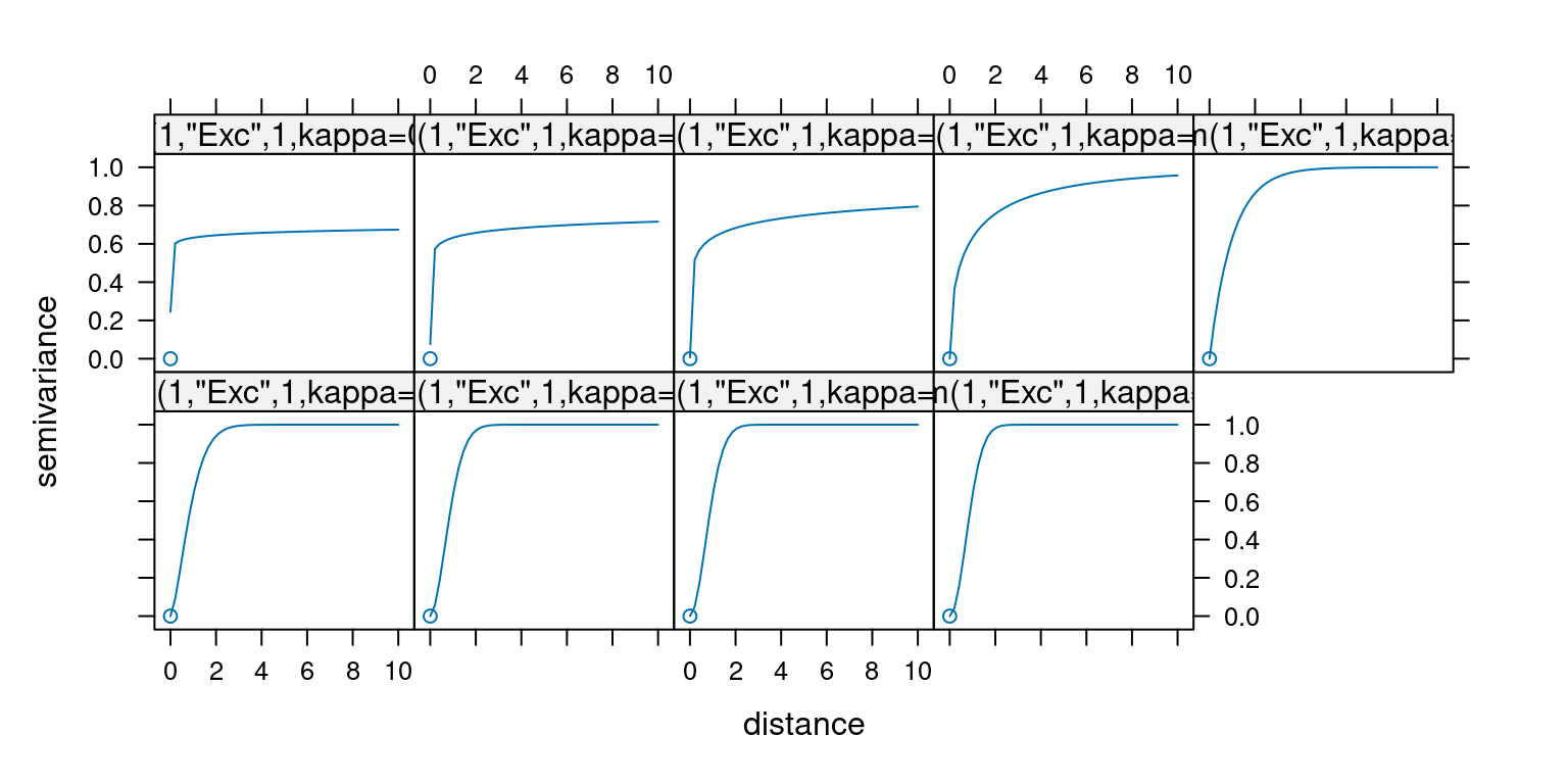
For the exponential variogram the effect of the shape parameter is as follows:
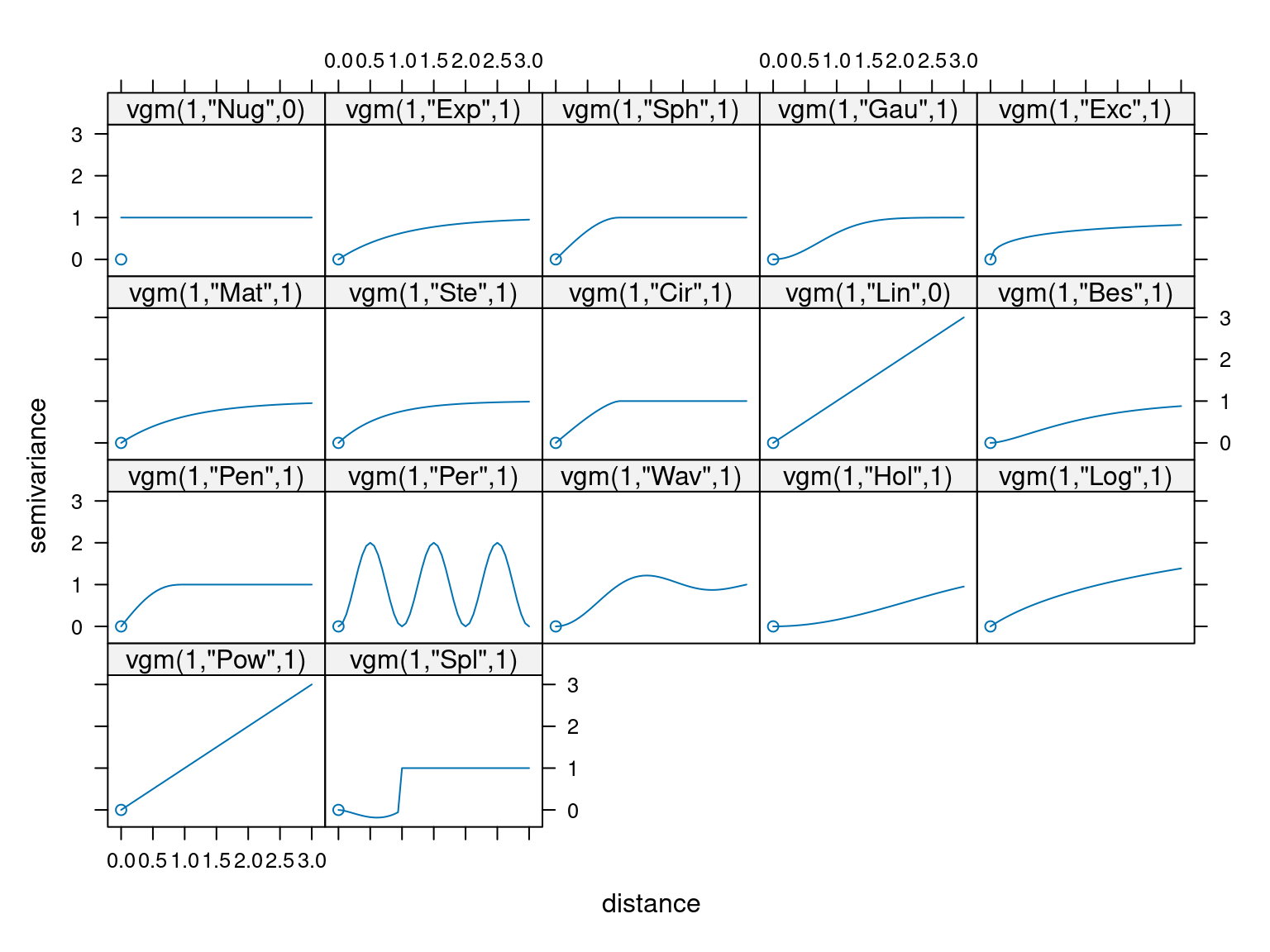
Other correlation functions / variograms exist but are used less often. The following plot shows all the variograms available in the gstat package in R:
 The long names of the abbreviations used in the plots can be looked up then calling
 vgm() without any arguments.
##    short                                      long
## 1    Nug                              Nug (nugget)
## 2    Exp                         Exp (exponential)
## 3    Sph                           Sph (spherical)
## 4    Gau                            Gau (gaussian)
## 5    Exc        Exclass (Exponential class/stable)
## 6    Mat                              Mat (Matern)
## 7    Ste Mat (Matern, M. Stein's parameterization)
## 8    Cir                            Cir (circular)
## 9    Lin                              Lin (linear)
## 10   Bes                              Bes (bessel)
## 11   Pen                      Pen (pentaspherical)
## 12   Per                            Per (periodic)
## 13   Wav                                Wav (wave)
## 14   Hol                                Hol (hole)
## 15   Log                         Log (logarithmic)
## 16   Pow                               Pow (power)
## 17   Spl                              Spl (spline)
## 18   Leg                            Leg (Legendre)
## 19   Err                   Err (Measurement error)
## 20   Int                           Int (Intercept)
Not all variograms level off with increasing distance - these are only used under special circumstances.
Typically the functions level off - the asymptote is called the sill and the distance at which the asymptote is reached is called the sill.
vgmPrediction <- variogramLine(vgm(psill = 20, model = "Sph", range=100), maxdist= 200)

ggplot(vgmPrediction, mapping=aes(x=dist,y=gamma)) + geom_line() +
  geom_hline(yintercept = 20, lty=3) +
    geom_vline(xintercept = 100, lty=3) +
  annotate("text", x=0, y=19.5, label= "sill") +
  annotate("text", x=110, y=5, label= "range") +
  xlab("Distance")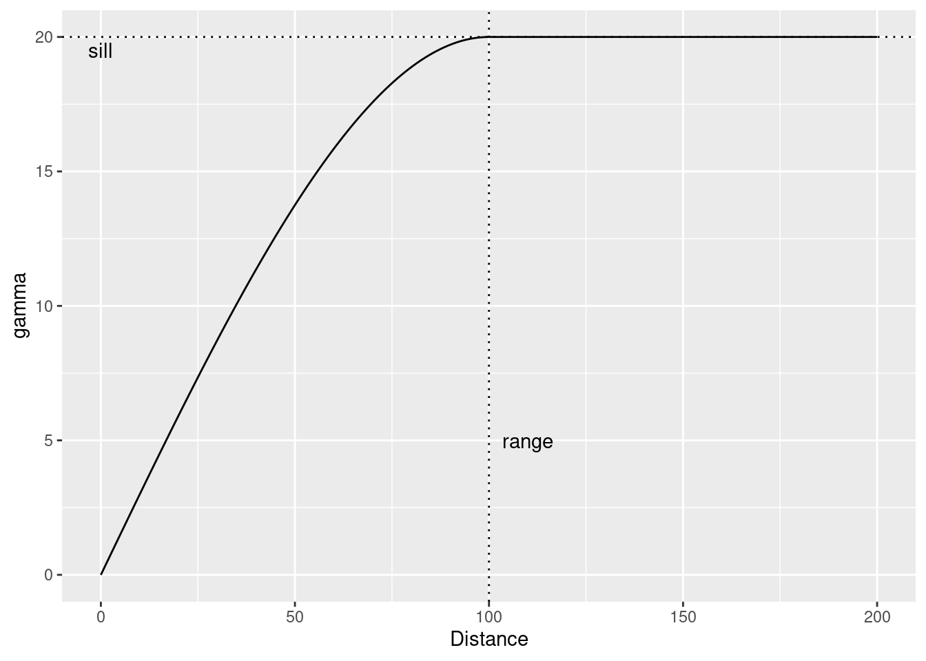
14.3.5 The nuggest effect
The nugget effect represents a discontinuity at the origin of the variogram. It can be interpreted as the measurement error variance.
vgmPrediction <- variogramLine(vgm(psill = 20, model = "Sph", range=100, nugget=5), maxdist= 200)

ggplot(vgmPrediction, mapping=aes(x=dist,y=gamma)) + geom_line() +
  geom_hline(yintercept = 20 +5, lty=3) +
   geom_hline(yintercept = 5, lty=3, col="brown") +
    geom_vline(xintercept = 100, lty=3) +
  annotate("text", x=0, y=24.5, label= "sill") +
  annotate("text", x=110, y=15, label= "range") +
  annotate("text", x=10, y=4.5, label= "nugget") +
  ylim(0,25) +
  xlab("Distance")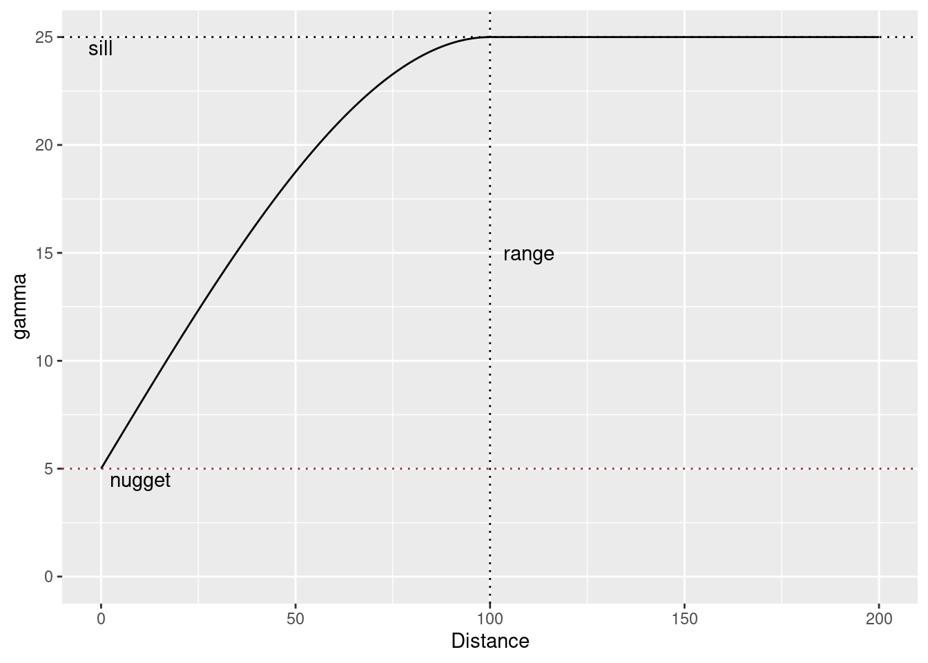
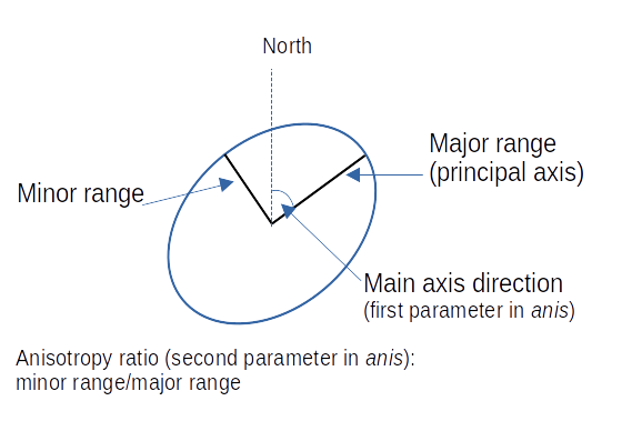
14.3.6 Anisotropy
If the correlation function does not only depend on distance between observations but also on the direction this is called anisotropy. The simplest form of directional effect on the covariance structure is geometrical anisotropy (different range). It can be modeled by using a range ellipse instead of a circular range. A model with geometrical anisotropy in spatial coordinates \((x_1,x_2)\) can be converted to a stationary model by transforming the coordinates in an appropriate way (Diggle and Ribeiro, 2007, p. 58) :
\[ (x_1', x_2') = \left[\begin{array} {rr} cos(\psi_A) & -sin(\psi_A) \\ sin(\psi_A) & cos(\psi_A) \end{array}\right] \left[\begin{array} {rr} 1 & 0 \\ 0 & cos(\psi_R) \end{array}\right] \]
where \(\psi_A\) is called the anisotropy angle and \(\psi_R\) is called the anisotropy ratio. The direction along which the correlation decays most slowly with increasing distance is called the principal axis.
In practice \(\psi_A\) and \(\psi_R\) are not known and have to be estimated from the data.
In gstat anisotropy can be modeled as part of the variogram specification (vgm). It is specified by two parameters for two dimensional data, which define an anisotropy ellipse, say anis = c(30, 0.5). The first parameter, 30, refers to the main axis direction (\(\psi_A\)): it is the angle for the principal direction of continuity (measured in degrees, clockwise from positive Y, i.e. North). The second parameter, 0.5, is the anisotropy ratio (\(\psi_R\)), the ratio of the minor range to the major range (a value between 0 and 1). So, in our example, if the range in the major direction (North-East) is 100, the range in the minor direction (South-East) is 0.5 x 100 = 50. The range estimated by fitting a variogram to the data is then defined as the range in the direction of the strongest correlation, or the major range. Anisotropy parameters define which direction this is (the main axis), and how much shorter the range is in (the) direction(s) perpendicular to this main axis.
In gstat it is currently not possible to estimate \(\psi_A\) and \(\psi_R\) from the data. One has to specify the values and try different combination and compare them e.g. by crossvalidation or by eyballing. Another option would be to use the package geoR which allows estimation of the parametres from the data using restricted maximum likelihood. 8
Zonal anisotropy (different sill) is more difficult to deal with.
14.3.7 Kriging
Kriging is a linear operator (similar to IDW) that predicts values of the target variable at unobserved location by a weighted sum of the observed values:
\[ \hat{z}(s_0) = \sum_{i=1}^n w_i \cdot z(s_i) \]
\[ \sum_{i=1}^n w_i = 1\]
The kriging weights \(w_i\) depend on the distance between the observations and the location for which we would like to estimate the target variable. The kriging weights are estimated based on the covariance matrix (which is “known” after we have fitted the theoretical variogram to the empirical variogram). For ordinary kriging the estimation is based on:
\[ w(s_0) = C^{-1}\cdot c_0\] where \(C\) is the covariance matrix for the \(n\) observations and \(c_0\) is the vector of covariances at the new location. Both \(C\) and \(c_0\) are “known” as they are based on the theoretical variogram fitted to the empirical variogram. This is how the (semi-) variogram is connected to the interpolation of new data.
\[ C(|h| = 0) = C_0 + C_1\] where \(C_0\) is the covariance of the nugget and \(C_0 + C_1\) is the covariance of the sill. \(C(h)\) is the covariance for the distance \(h\).
\[C(|h| > 0) = C_1*\rho(h)\]
More specifically, \(C\) is the n x n covariance matrix extended by one row and one columns to allow solving the equation system. This last row and column ensures the constraint that the weights sum up to unity.
\[ \left[\begin{array} {c} w_1(s_0)\\ \vdots \\ w_n(s_0)\\ \xi \end{array}\right] = \left[\begin{array} {cccc} C(s_1,s_1) & \ldots & C(s_1,s_n) & 1 \\ \vdots & \vdots & \vdots & \vdots \\ C(s_n,s_1) & \ldots & C(s_n,s_n) & 1 \\ 1 & \ldots & 1 & 0 \end{array}\right]^{-1} \cdot \left[\begin{array} {c} C(s_0,s_1)\\ \vdots \\ C(s_0,s_n)\\ 1 \end{array}\right] \]
where \(\xi\) is the Lagrange multiplier.
The weights can then be used for the prediction. In addition to the prediction, kriging also provides information about the uncertainty of the prediction at each location for which we asked for a prediction. This is often called the prediction variance, its square root can be thought of as the standard error of the prediction. For ordinary kriging, the prediction variance is defined as the weighted average of covariances for the location to be predicted (\(s_0\)) to all observations \((s_1, \ldots, s_n)\), plus the Lagrange multiplier:
\[ \hat{\sigma}_{OK}^2 = C_0 + C_1 - \sum_{i=1}^n w_i(s_0) \cdot C(s_0,s_i) + \xi\]
In contrast to simpler approaches such as IDW, kriging weights can be negative and larger than one, as long as they sum up to unity.
The kriging terminology distinguishes some special cases. While this sounds overly complex, it is straightforward to use the different variants ingstat.
- ordinary kriging: no regression parameters beside the intercept have to be estimated, e.g. we assume that \(S(X)\) can be described as fluctuations around the mean
- simple kriging: we assume that we - or whatever reasons - know the mean and are able to provide it. Therefore, the mean (intercept) does not have to be estimated from the data
- universal kriging: we assume an effect by covariates and a spatial trend that needs to be taken into account by modelling that
- kriging with external drift: similar to universal kriging but we assume no spatial trend - i.e. the coordinates are not used in the regression formula
In gstat all variants are modeled with krige() (or gstat(). The function is smart enough to figure out which version we mean from the parameters we provide.
14.3.7.1 Kriging step by step
I hope it is helpful to examine the kriging process for a small sample. We follow the example provided by (Isaaks and Srivastava, 1989). The example consists of just seven observations and demonstrates interpolation for a single location (id=99):
dat <- data.frame(
  id = c(1:7,99),
  X = c(61,63,64,68,71,73,75, 65),
  Y = c(139,140,129,128,140,141,128, 137),
  V = c(477,696,227,646,606,791,783,NA),
  type = c(rep("obs",7), "predict")
)ggplot(dat, aes(x=X, y=Y, colour=type, label=V)) +
geom_point(show.legend = FALSE) +
xlab("") + ylab("") +
geom_text(nudge_y = 1, show.legend = FALSE)## Warning: Removed 1 row containing missing values or values outside the scale range
## (`geom_text()`).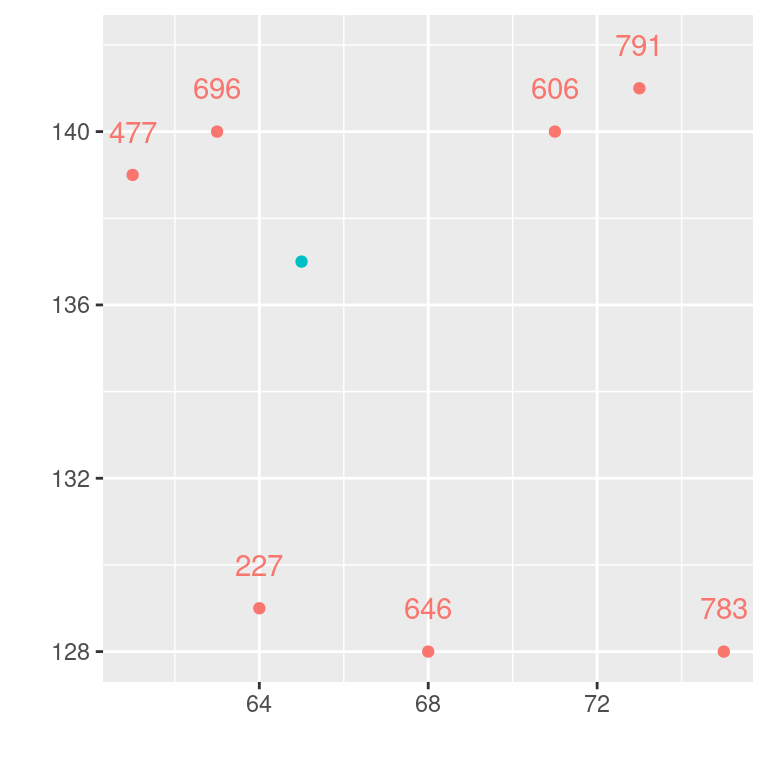
We need the distance between the observations and the location to be interpolated. This can be done by using the euclidian distance formula.
The calculation of the kriging weights depends on the covariance function. We start with the following covariance function:
\[ \tilde{C}(h) = \left \{ \begin{array} {ll} C_0 + C_1 & if |h| =0 \\ C_1 \cdot e^{\frac{-3|h|}{a}} & if |h| >0 \end{array}\right. \]
Which corresponds to the following variogram:
\[ \tilde{\gamma}(h) = \left \{ \begin{array} {ll} 0 & if |h| =0 \\ C_0 + C_1 \cdot (1- e^{\frac{-3|h|}{a}}) & if |h| >0 \end{array}\right. \]
Where \(C_0\) is the nugget effect, \(C_0 + C_1\) the sill and \(a\) the range (see above).
For demonstration purpose we will set the parameters as follows:
\[ \begin{array} {lll} C_0 = 0, & a= 10, & C_1 = 10 \end{array}\]
This leads to the following covariance model:
\[ \tilde{C}(h) = 10 e^{-0.3|h|} \]
myC <- function(h, C0=0, C1=10, a=0.3){
  res <- ifelse(h==0,
                C0 + C1,
                C1*exp(-a*abs(h))  )
  return(res)
}
The corresponding variogram function
myVariogram <- function(h, C0=0, C1=10, a=0.3){
  res <- ifelse(h ==0,
                C0,
                C0 + C1*(1-exp(-a*abs(h))))
  return(res)
} ggplot() + geom_function(fun=myC) + xlim(0,20) +
geom_function(fun=myVariogram, lty=2) +
ylab("Covariance or Variance") +
xlab("Distance (h)") +
labs(title = "Covariance (bold) and variance (dashed)",
subtitle = "For C0 = 0, C1 = 10 and a = 0.3")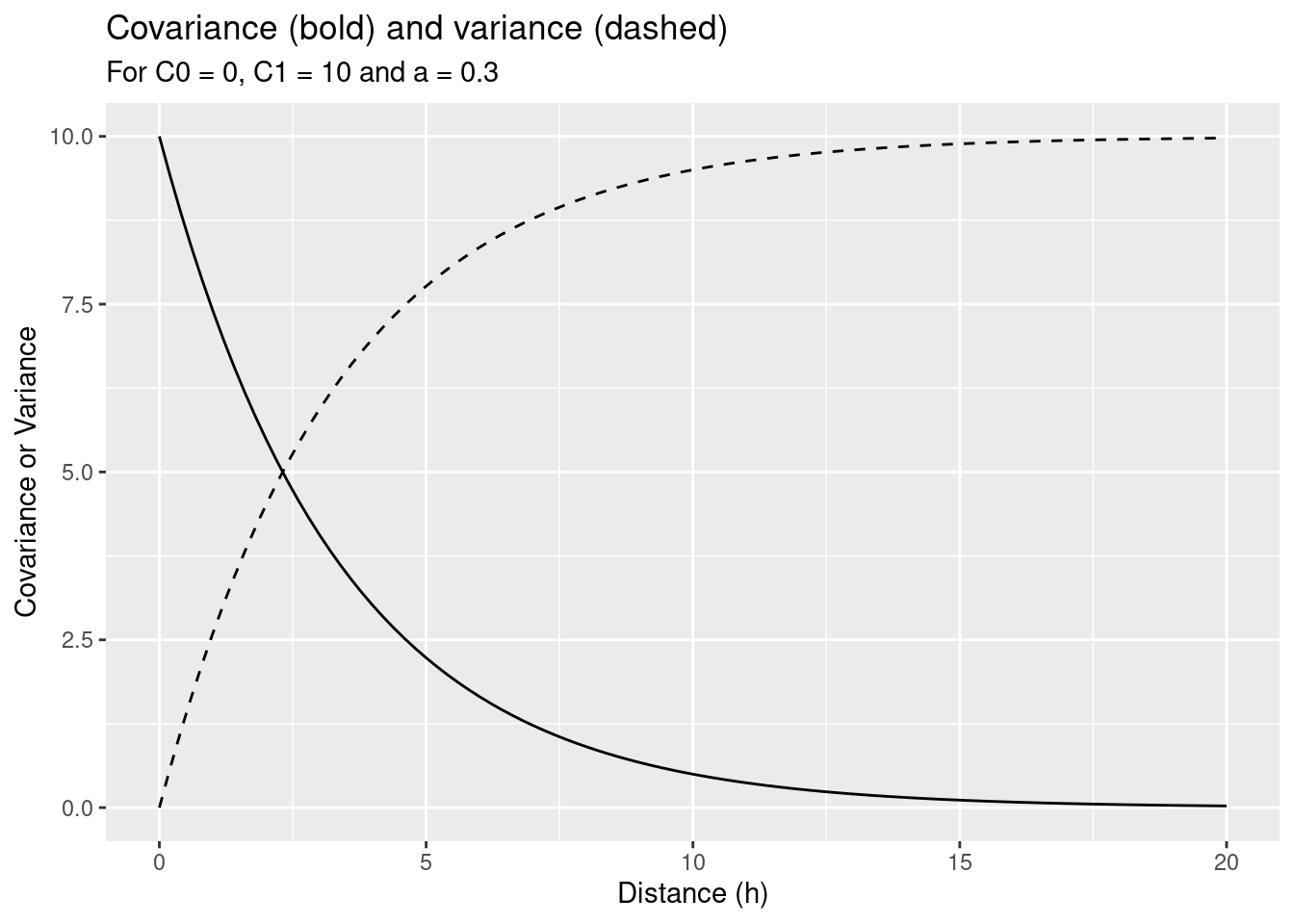
After calculating the distances between all our observations, we can calculate the matrices \(C\) and \(c_0\).
obsSf <- dat %>%
    st_as_sf(coords = c("X", "Y") )
st_distance(obsSf, which = "Euclidean") %>%
   round(2) %>%
knitr::kable(caption="Distances between locations")| 1 | 2 | 3 | 4 | 5 | 6 | 7 | 8 |
|---|---|---|---|---|---|---|---|
| 0.00 | 2.24 | 10.44 | 13.04 | 10.05 | 12.17 | 17.80 | 4.47 |
| 2.24 | 0.00 | 11.05 | 13.00 | 8.00 | 10.05 | 16.97 | 3.61 |
| 10.44 | 11.05 | 0.00 | 4.12 | 13.04 | 15.00 | 11.05 | 8.06 |
| 13.04 | 13.00 | 4.12 | 0.00 | 12.37 | 13.93 | 7.00 | 9.49 |
| 10.05 | 8.00 | 13.04 | 12.37 | 0.00 | 2.24 | 12.65 | 6.71 |
| 12.17 | 10.05 | 15.00 | 13.93 | 2.24 | 0.00 | 13.15 | 8.94 |
| 17.80 | 16.97 | 11.05 | 7.00 | 12.65 | 13.15 | 0.00 | 13.45 |
| 4.47 | 3.61 | 8.06 | 9.49 | 6.71 | 8.94 | 13.45 | 0.00 |
We get the matrix \(C\) simply by evaluating the previously defined covariance function for the distances between the pairs and augmenting it by the additional row and column to add the constraint (weights sum up to unity).
| 1 | 2 | 3 | 4 | 5 | 6 | 7 |
|---|---|---|---|---|---|---|
| 10.000 | 5.113 | 0.436 | 0.200 | 0.490 | 0.260 | 0.048 |
| 5.113 | 10.000 | 0.364 | 0.202 | 0.907 | 0.490 | 0.062 |
| 0.436 | 0.364 | 10.000 | 2.903 | 0.200 | 0.111 | 0.364 |
| 0.200 | 0.202 | 2.903 | 10.000 | 0.245 | 0.153 | 1.225 |
| 0.490 | 0.907 | 0.200 | 0.245 | 10.000 | 5.113 | 0.225 |
| 0.260 | 0.490 | 0.111 | 0.153 | 5.113 | 10.000 | 0.193 |
| 0.048 | 0.062 | 0.364 | 1.225 | 0.225 | 0.193 | 10.000 |
Now we add the row and column that represent the constraint.
| 1 | 2 | 3 | 4 | 5 | 6 | 7 | ||
|---|---|---|---|---|---|---|---|---|
| 1 | 10.000 | 5.113 | 0.436 | 0.200 | 0.490 | 0.260 | 0.048 | 1 |
| 2 | 5.113 | 10.000 | 0.364 | 0.202 | 0.907 | 0.490 | 0.062 | 1 |
| 3 | 0.436 | 0.364 | 10.000 | 2.903 | 0.200 | 0.111 | 0.364 | 1 |
| 4 | 0.200 | 0.202 | 2.903 | 10.000 | 0.245 | 0.153 | 1.225 | 1 |
| 5 | 0.490 | 0.907 | 0.200 | 0.245 | 10.000 | 5.113 | 0.225 | 1 |
| 6 | 0.260 | 0.490 | 0.111 | 0.153 | 5.113 | 10.000 | 0.193 | 1 |
| 7 | 0.048 | 0.062 | 0.364 | 1.225 | 0.225 | 0.193 | 10.000 | 1 |
| 1.000 | 1.000 | 1.000 | 1.000 | 1.000 | 1.000 | 1.000 | 0 |
The n+1 x 1 matrix \(c_0\) is calculated by evaluating the covariance function for the distances between the observations and the new location and adding the additional row:
## [1] 2.6141639 3.3903044 0.8903931 0.5807326 1.3365931 0.6833853 0.1766646
## [8] 1.0000000
Next we can calculate the inverse of \(C\) - remember that \(C * C^{-1} = I\) there \(I\) is the identity matrix.
| 1 | 2 | 3 | 4 | 5 | 6 | 7 | ||
|---|---|---|---|---|---|---|---|---|
| 1 | 0.127 | -0.077 | -0.013 | -0.009 | -0.008 | -0.009 | -0.012 | 0.136 |
| 2 | -0.077 | 0.129 | -0.010 | -0.008 | -0.015 | -0.008 | -0.011 | 0.121 |
| 3 | -0.013 | -0.010 | 0.098 | -0.042 | -0.010 | -0.010 | -0.014 | 0.156 |
| 4 | -0.009 | -0.008 | -0.042 | 0.102 | -0.009 | -0.009 | -0.024 | 0.139 |
| 5 | -0.008 | -0.015 | -0.010 | -0.009 | 0.130 | -0.077 | -0.012 | 0.118 |
| 6 | -0.009 | -0.008 | -0.010 | -0.009 | -0.077 | 0.126 | -0.013 | 0.141 |
| 7 | -0.012 | -0.011 | -0.014 | -0.024 | -0.012 | -0.013 | 0.085 | 0.188 |
| 0.136 | 0.121 | 0.156 | 0.139 | 0.118 | 0.141 | 0.188 | -2.180 |
Now we can calculate the kriging weights, simply by a matrix multiplication between \(C^{-1}\) and \(c_0\):
\(w = C^{-1} * c_0\)
##          [,1]
## 1  0.17293732
## 2  0.31779357
## 3  0.12873406
## 4  0.08639657
## 5  0.15112770
## 6  0.05723465
## 7  0.08577613
##   -0.90661662
The first seven elements in w are the kriging weights, the last one is the Lagrange multiplier.
Estimation of V at the new location:
##          [,1]
## [1,] 592.7289
dat1 <- dat
dat1$w <- c(w[1:7], NA)
ggplot(dat1, aes(x=X, y=Y, colour=type, label= round(w,2))) +
geom_point(show.legend = FALSE) +
xlab("") + ylab("") + labs(title = "kriging weights") +
geom_text(nudge_y = 1, show.legend = FALSE) +
geom_text(mapping= aes(label=id), colour="black",
nudge_y = 0.5, show.legend = FALSE,
fontface = "italic")## Warning: Removed 1 row containing missing values or values outside the scale range
## (`geom_text()`).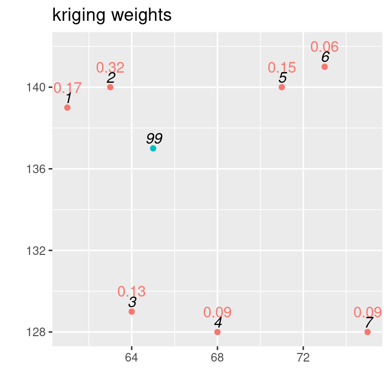
Figure 14.1: IDs in black, kriging weights coloured
The estimated variance is calculated as:
\[ \tilde{\sigma}^2_R = \tilde{\sigma}^2 - \sum_{i=1}^n w_i \tilde{C}_{i0} + \mu \]
with \(\tilde{\sigma}^2\) the covariance for h=0, \(w_i\) the kriging weights, \(\tilde{C}_{i0}\) the covariance matrix for the new location and \(\mu\) the Lagrange parameter.
In our example
\(\tilde{\sigma}^2\):
## [1] 10\(\mu\):
## [1] -0.9066166\(\tilde{\sigma}^2_R\):
## [,1]
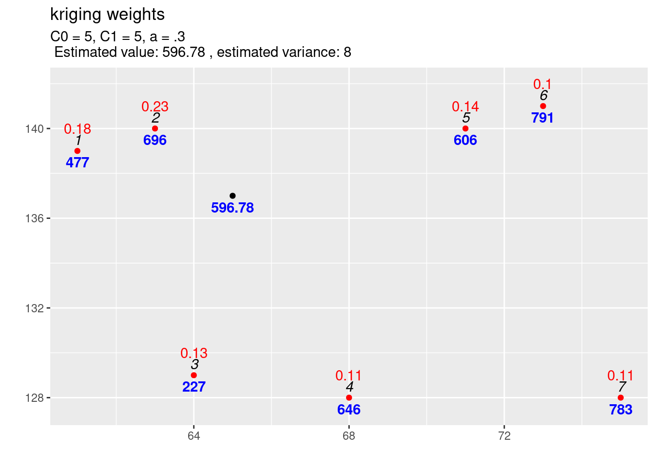
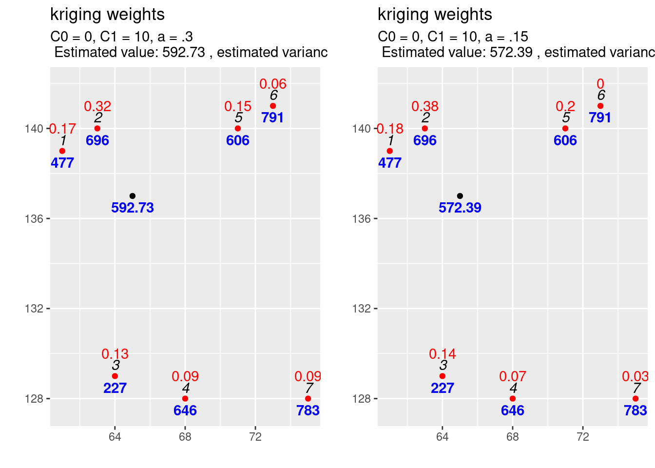
## [1,] 7.14282To get a better idea how kriging works and how the weights assigned by it differ from approaches such as IDW, it is helpful to inspect the kriging weights in figure \(ref?)(fig:exampleKW1). Let’s take a look at observation with the ID 4 and 6. The observation with ID 4 is further away than the observation with ID 6. So for weights assigned based on distance we would expect that the observation with ID 6 would get a higher weight. This is, however, not the case for our example. Kriging uses the full covariance matrix, that is based on the distances between the observations and the location to be interpolated as well as between the observations. As the observation with the IDs 5 and 6 are close to each other (clustered), this is taken into account then solving the equation for the kriging weights. Kriging thereby solves for the issue of clustered observations, that approaches such as IDW fall for.
The covariance matrix \(c0\) reflects that observation with ID 6 is closer than ID 4 to the location to be interpolated as the covariance with the new location for ID 6 is higher than for ID 4.
## [1] 0.5807326## [1] 0.6833853For the kriging weights this is different due to the matrix multiplication with \(C^{-1}\).
## [1] 0.08639657## [1] 0.05723465To observations close to each other will result in a large value in the covariance matrix \(C\).
## [1] 5.112889This is a large value compared to the other values in the covariance matrix. Keep in mind that 10 is the variance at distance 0.
##    Min. 1st Qu.  Median    Mean 3rd Qu.    Max.
##  0.0000  0.2024  0.4905  1.9158  1.0000 10.0000
Clustering is represented in \(C^{-1}\) while distances between observations and the location to be interpolated is represented in \(c0\):
\[ w = C^{-1} \cdot c_0 \]
The kriging weights are specific for the location to be interpolated. If we chose a different location for the interpolation, \(c_0\) would change and thereby \(w\). \(C\) and \(C^{-1}\) would not change as these capture the relationship between the observations which are fixed.9
14.3.7.1.0.1 Helper functions
To avoid redundant code, I have put everything into a function that performs the required calculations, creates the plot and returns the plot together with the kriging weights. To make the function more flexible, I use a design pattern known as function factory. Based on a generic function for the exponential covariance family the function factory creates a function for which the parameters beside distance (h) are set. The benefit is that I can use the model for different functions, even if those require different parameters.
expCovFactory <- function(C0, C1, a)
{
  function(h)
    {
      res <- ifelse(h==0,
                C0 + C1,
                C1*exp(-a*abs(h))  )
      return(res)
  }
}
calcKrigingWeights <- function(observations, newlocation, covfun,
text4plot = "", plotit = TRUE, verbose=FALSE)
{
n <- nrow(observations)
# distances between observations and new location
dist2loc <- sqrt((observations$X-newlocation$X)^2 + (observations$Y-newlocation$Y)^2)
# distances between observations
obsDist <- observations %>%
st_as_sf(coords = c("X", "Y") ) %>%
st_distance(which = "Euclidean")
# covariance matrix for observations
Cmat <- covfun(obsDist)
# add Lagrange multiplier
Cmat <- cbind(Cmat, rep(1,7)) %>%
rbind(c(rep(1,7),0))
# invert C
CmatInv <- solve(Cmat)
# covariance between obs and new locations
c0 <- covfun(dist2loc) %>% c(1)
# kriging weights
w <- CmatInv %*% c0
kw <- w[1:n]
lagmult <- w[n+1]
# prediction
thePrediction <- kw %*% observations$V
# estimated variance
estVar <- covfun(0) - kw %*% c0[1:n] + w[n+1]
resStr <- paste("Estimated value:", round(thePrediction,2),
", estimated variance:", round(estVar,2) )
if(verbose)
cat(paste(resStr, "\n"))
# create plot
p1 <- ggplot(observations, aes(x=X, y=Y, label= round(kw,2))) +
geom_point(show.legend = FALSE, colour = "red") +
xlab("") + ylab("") +
labs(title = "kriging weights", subtitle = paste(text4plot, "\n", resStr)) +
geom_text(nudge_y = 1, show.legend = FALSE, colour = "red") +
geom_text(mapping= aes(label=id), colour="black",
nudge_y = 0.5, show.legend = FALSE,
fontface = "italic") +
geom_text(mapping= aes(label=V), colour="blue",
nudge_y = -0.5, show.legend = FALSE,
fontface = "bold") +
geom_point(data= newlocation, mapping=
aes(x=X, y=Y ), show.legend = FALSE,
inherit.aes = FALSE) +
geom_text(data= newlocation, mapping= aes(label=round(thePrediction,2)), colour="blue",
nudge_y = -0.5, show.legend = FALSE,
fontface = "bold")
if(plotit)
print(p1)
return(list(krigingweigts = kw, lagrangeMultiplier = lagmult, kwplot = p1))
}With that functions it is easy to study the effect of a new location on the kriging weights (cf. figure 14.2).
newlocation_b <- data.frame(id=100, X=73, Y = 129, V=NA)

observations <- dat[1:7, 1:4]
newlocation <- dat[8, 1:4]

expCov_0_10_03 <- expCovFactory(C0 = 0, C1 = 10, a=0.3)

kw1_b <- calcKrigingWeights(observations, newlocation_b, covfun= expCov_0_10_03,
                   text4plot = "C0 = 0, C1 = 10, a = .3", plotit=FALSE)

kw1_b$kwplot +
  annotate(geom="label", x=73, y=130.2,
           label="interpolated point")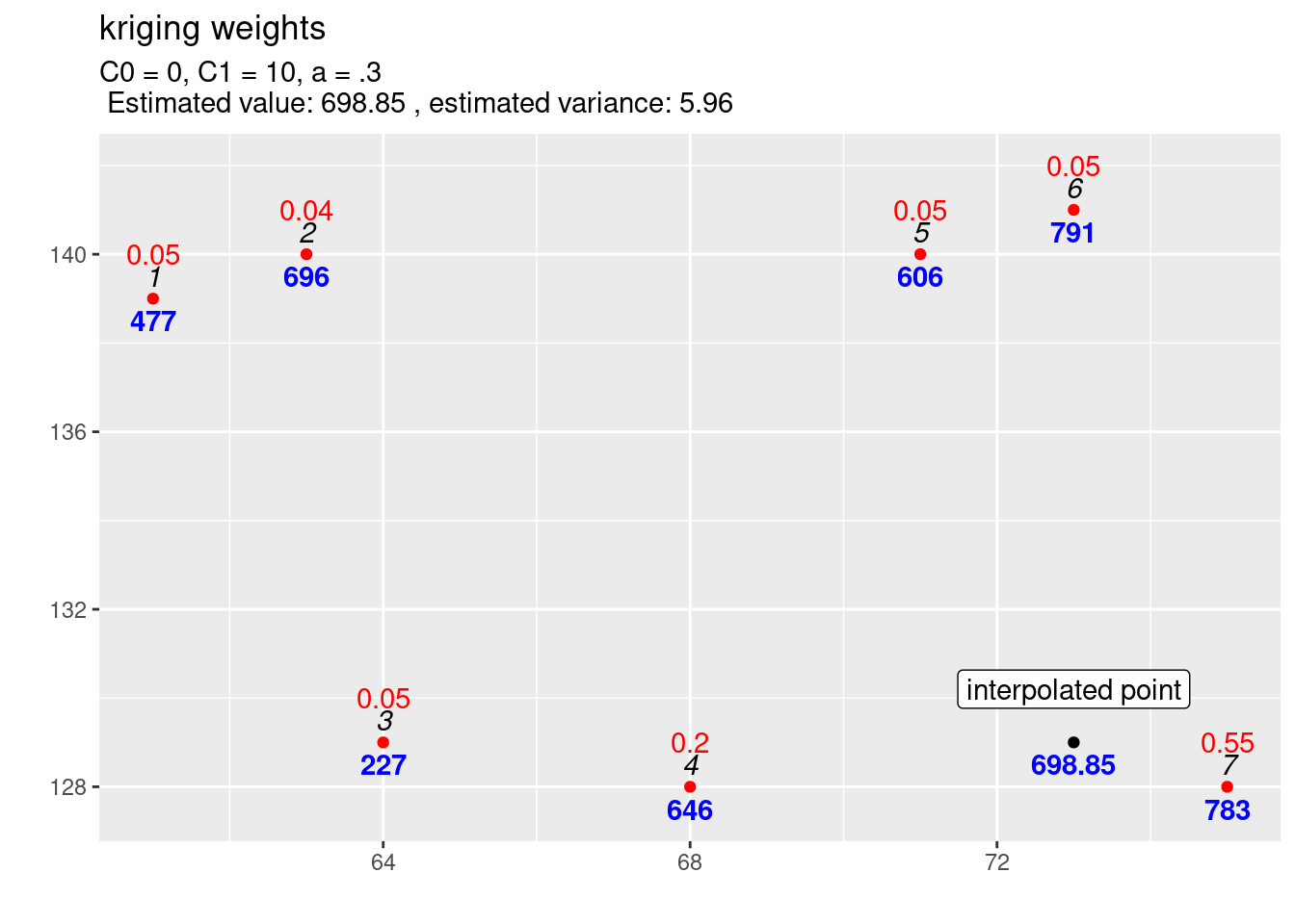
Figure 14.2: Kriging weights (red) and interpolated value for a different location. The blues numbers indicate the observed (or predicted) values, the black italic numbers the id of the location and the red numbers the kriging weights for the selected location for which the estimation is performed.
Lets compare with the previous unobserved location (cf. figure 14.3): kriging weights, interpolated value and uncertainty of the estimation all changed as expected.
kw1 <- calcKrigingWeights(observations, newlocation, covfun= expCov_0_10_03,
                   text4plot = "C0 = 0, C1 = 10, a = .3", plotit=FALSE)

kw1$kwplot +
  annotate(geom="label", x=66.5, y=138,
           label="interpolated point")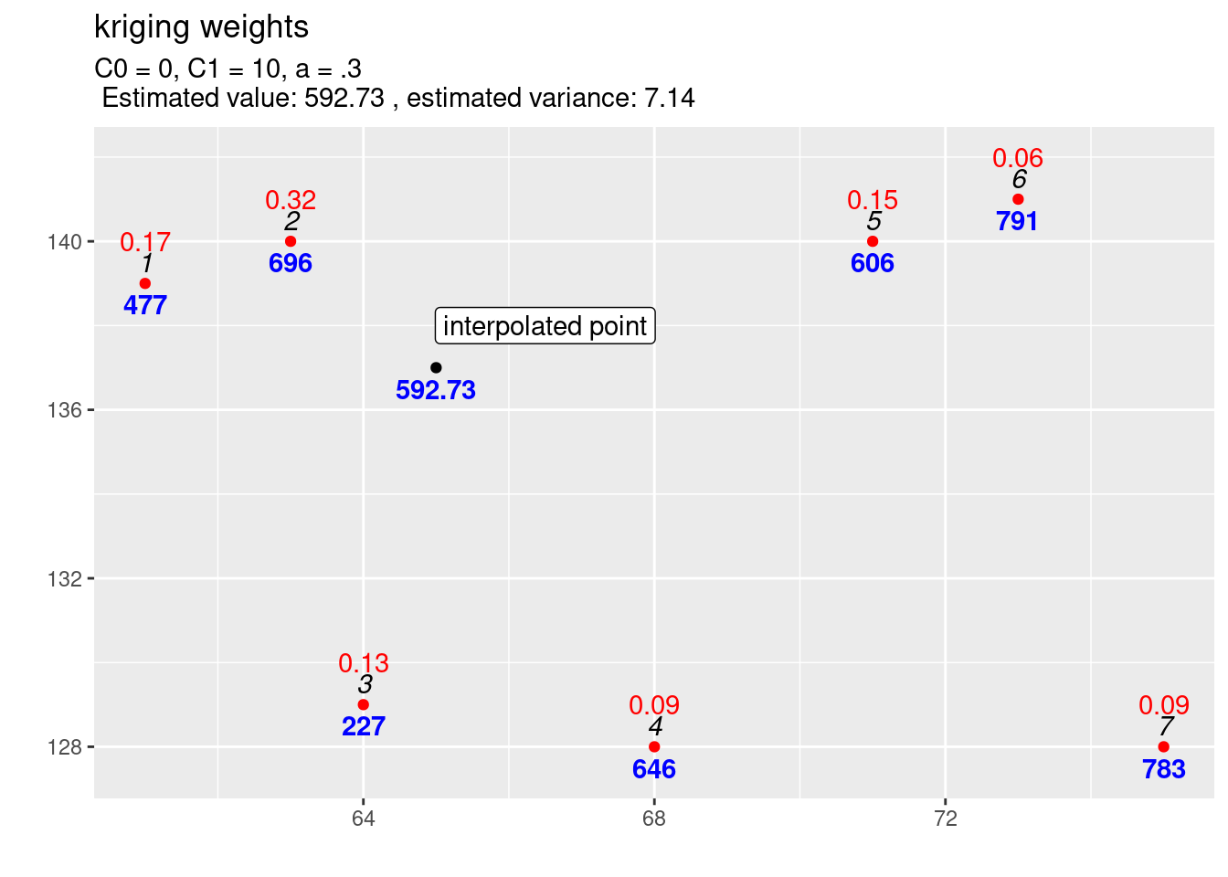
Figure 14.3: Kriging weights (red) and interpolated value for the first location. The blues numbers indicate the observed (or predicted) values, the black italic numbers the id of the location and the red numbers the kriging weights for the selected location for which the estimation is performed.
14.3.7.1.1 The effect of changing the scale parameter
If we change the scale parameter C1 from 10 to 20 for the exponential function defined above this results in an obvious increase of the variance for distances \(h>0\) (cf. figure 14.4). What might be the effects on the interpolated value, the kriging weights and the uncertainty of the predicted (interpolated) value at the unobserved location?
params0 <- list(C0=0, C1=10, a=.3)
params <- list(C0=0, C1=20, a=.3)
ggplot() + geom_function(fun=myC, args= params) + xlim(0,20) +
  geom_function(fun=myVariogram, lty=2, args= params) +
  geom_function(fun=myC, args= params0, col="blue")  +
  geom_function(fun=myVariogram, lty=2, args= params0, col= "blue") +
  ylab("Covariance or Variance") +
  xlab("Distance (h)") +
  labs(title = "Covariance (bold) and variance (dashed)",
       subtitle = "For C0 = 0, C1 = 20 and a = 0.3 (black) and C0 = 0, C1 = 10 and a = 0.3 (blue)")+
  annotate(geom="label", x=12, y=17.4,
           label="C1=20") +
  annotate(geom="label", x=12, y=7.3,
           label="C1=10", col="blue")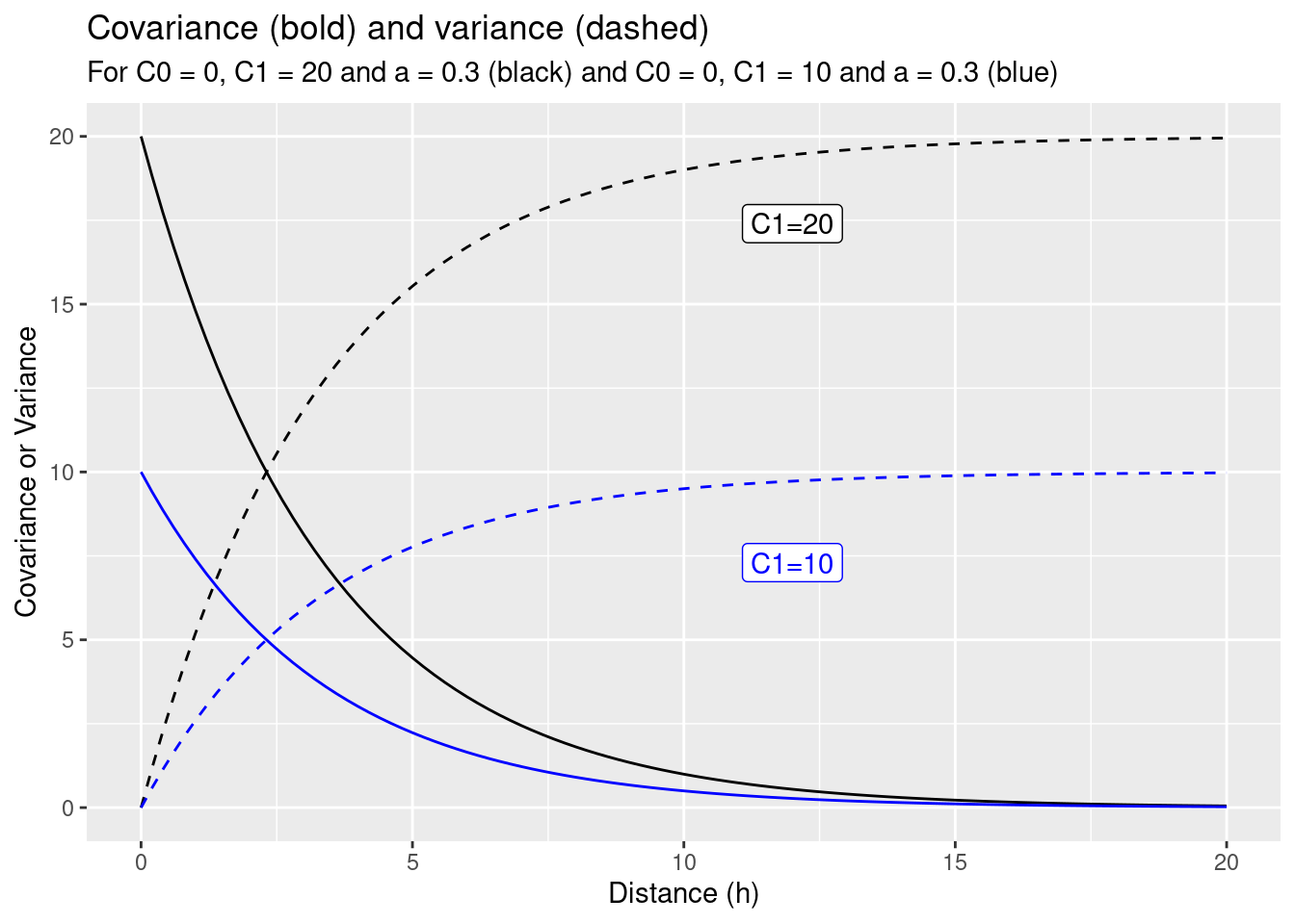
Figure 14.4: Effect of changing the scale parameter C1 from 10 (blue) to 20 (black) for the toy example.
observations <- dat[1:7, 1:4]
newlocation <- dat[8, 1:4]
expCov_0_20_03 <- expCovFactory(C0 = 0, C1 = 20, a=0.3)

kw2 <- calcKrigingWeights(observations = observations,
                          newlocation = newlocation,
                          covfun= expCov_0_20_03,
                          text4plot = "C0 = 0, C1 = 20, a = .3")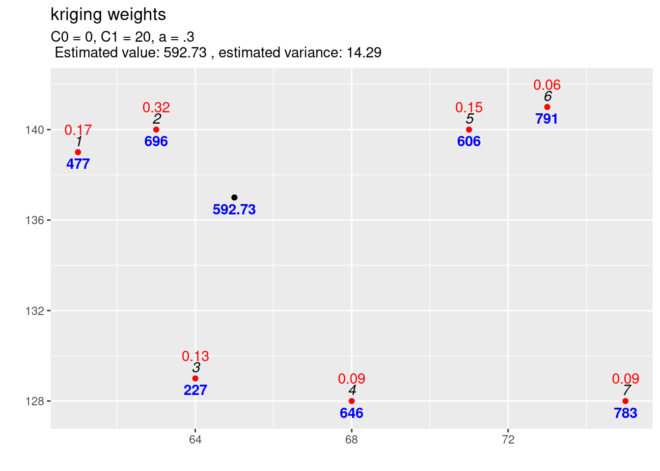
Figure 14.5: Kriging weights (red) and interpolated value for the first location. The blues numbers indicate the observed (or predicted) values, the black italic numbers the id of the location and the red numbers the kriging weights for the selected location for which the estimation is performed. Compared to the reference function the scale parameter has been increased from C1=10 to C1=10.
If we compare the interpolation for the increased scale parameter (cf. figure 14.5) with the results for the previous covariance function (cf. figure 14.6) we observe differences: The estimated value is exactly the same, but the estimated variance has increased. This is what always happens if we increase the scale (\(C_1\)) only: the estimation is unchanged but the variance of the estimation gets larger if the scale parameter is getting higher. A higher covariance between observations and new location leads to higher uncertainty of the estimation. The kriging weights did not change as well (otherwise we should have gotten a different estimate).
expCov_0_10_03 <- expCovFactory(C0 = 0, C1 = 10, a=0.3)
kw1 <- calcKrigingWeights(observations, newlocation, covfun= expCov_0_10_03,
                   text4plot = "C0 = 0, C1 = 10, a = .3")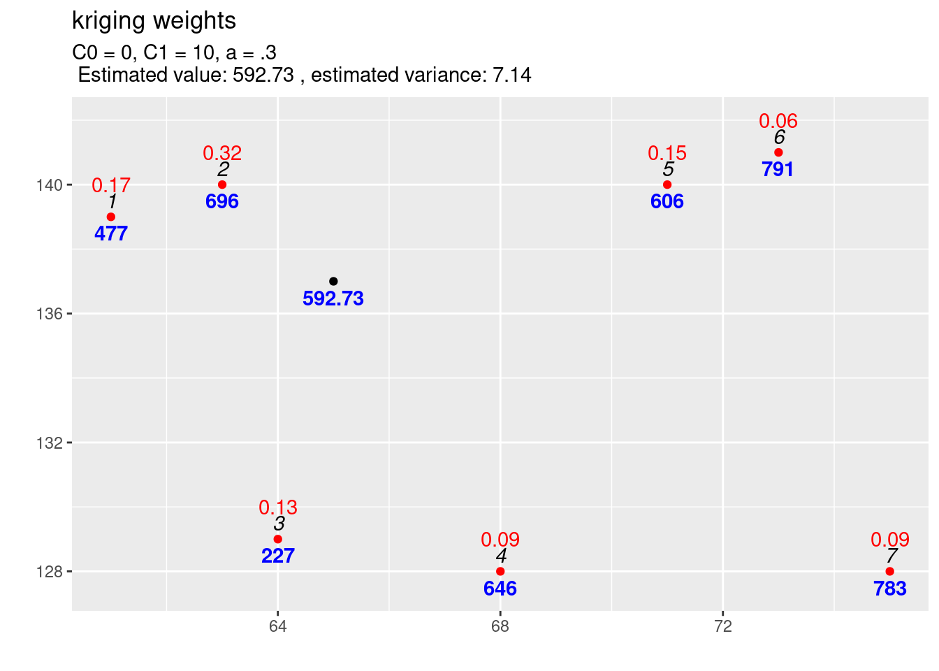
Figure 14.6: Interpolation results for the reference parametrisation for the exponential variogram function.
14.3.7.1.2 The effect of changing the nugget parameter
Next, we study the effects induced by adding a nugget effect but keeping the sill constant.
params0 <- list(C0=0, C1=10, a=.3)
params <- list(C0=5, C1=5, a=.3)
expCov_5_5_03 <- expCovFactory(C0 = 5, C1 = 5, a=0.3)
ggplot() + geom_function(fun=expCov_5_5_03) + xlim(0,20) +
  geom_function(fun=myVariogram, lty=2, args= params) +
  geom_function(fun=expCov_0_10_03,  col="blue")  +
  geom_function(fun=myVariogram, lty=2, args= params0, col= "blue") +
  ylab("Covariance or Variance") +
  xlab("Distance (h)") +
  labs(title = "Covariance (bold) and variance (dashed)",
       subtitle = "For C0 = 5, C1 = 5 and a = 0.3 (black) and C0 = 0, C1 = 10 and a = 0.3 (blue)")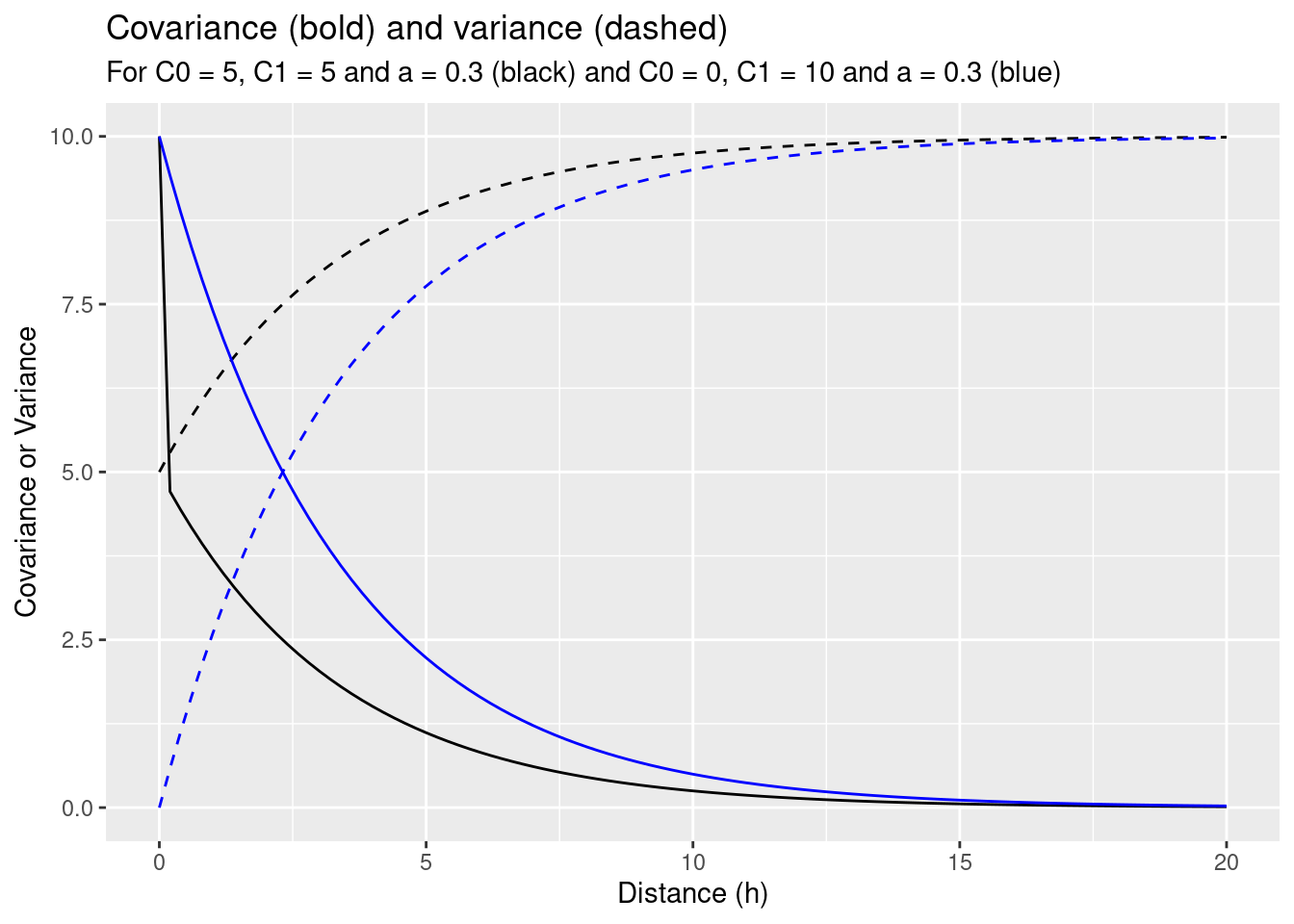
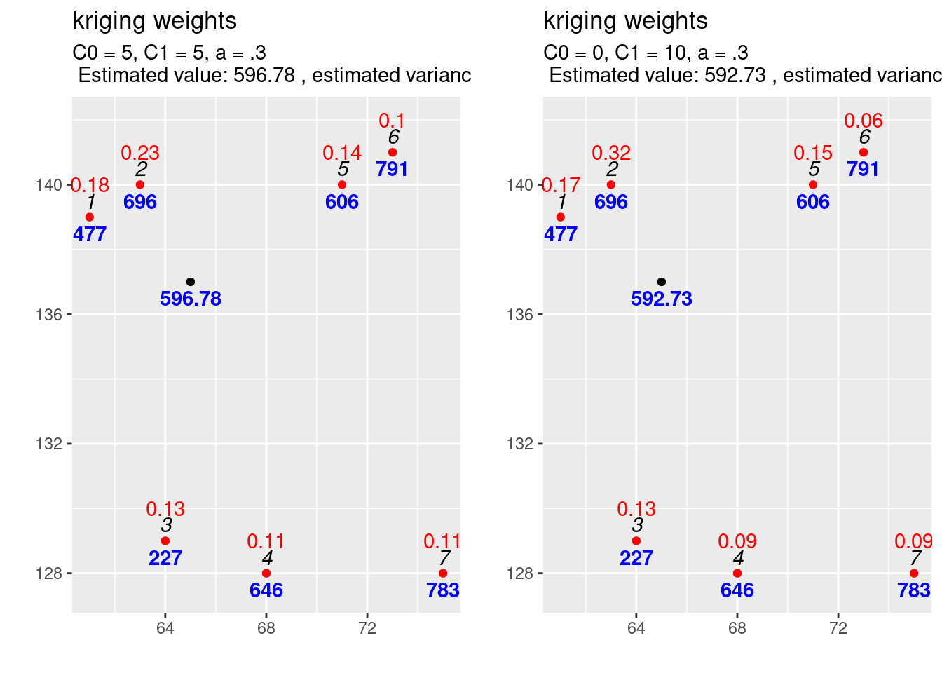
kw3 <- calcKrigingWeights(observations, newlocation, covfun= expCov_5_5_03,
                   text4plot = "C0 = 5, C1 = 5, a = .3"
                  )
Inclusion of the nugget effect has led to a change in prediction. The variance of the estimation increased compared to the model with the same sill but without a nugget effect. We see, that the kriging weights have changed and are now more similar to each other. This is a result of the nugget effect which implies, that for short distances the correlation between point pairs is lower, leading to a reduction of weights for those observations closer to the new location.
14.3.7.1.3 The effect of changing the range parameter
Next we explore the effect of increasing the range for the same sill and nugget effect.
expCov_0_10_015 <- expCovFactory(C0 = 0, C1 = 10, a=0.15)

params0 <- list(C0=0, C1=10, a=.3)
params <- list(C0=0, C1=10, a=.15)
ggplot() + geom_function(fun=expCov_0_10_015) + xlim(0.001,20) +
  geom_function(fun=myVariogram, lty=2, args= params) +
  geom_function(fun=expCov_0_10_03, col="blue")  +
  geom_function(fun=myVariogram, lty=2, args= params0, col= "blue") +
  ylab("Covariance or Variance") +
  xlab("Distance (h)") +
  labs(title = "Covariance (bold) and variance (dashed)",
       subtitle = "For C0 = 0, C1 = 10 and a = 0.15 (black) and C0 = 0, C1 = 10 and a = 0.3 (blue)")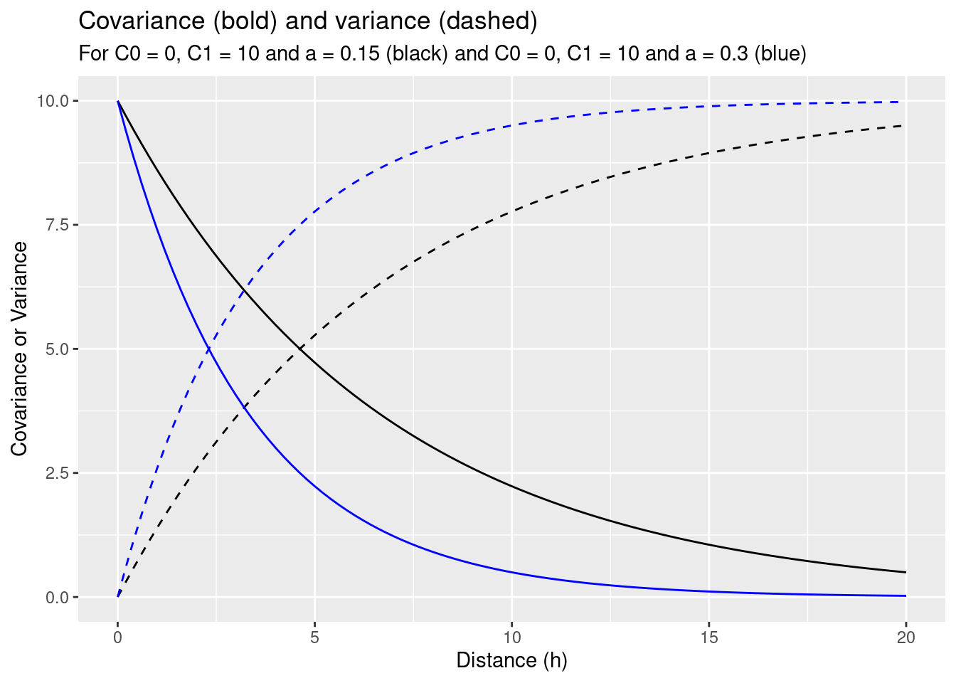
kw4 <- calcKrigingWeights(observations, newlocation, covfun = expCov_0_10_015,
                   text4plot = "C0 = 0, C1 = 10, a = .15"
                  )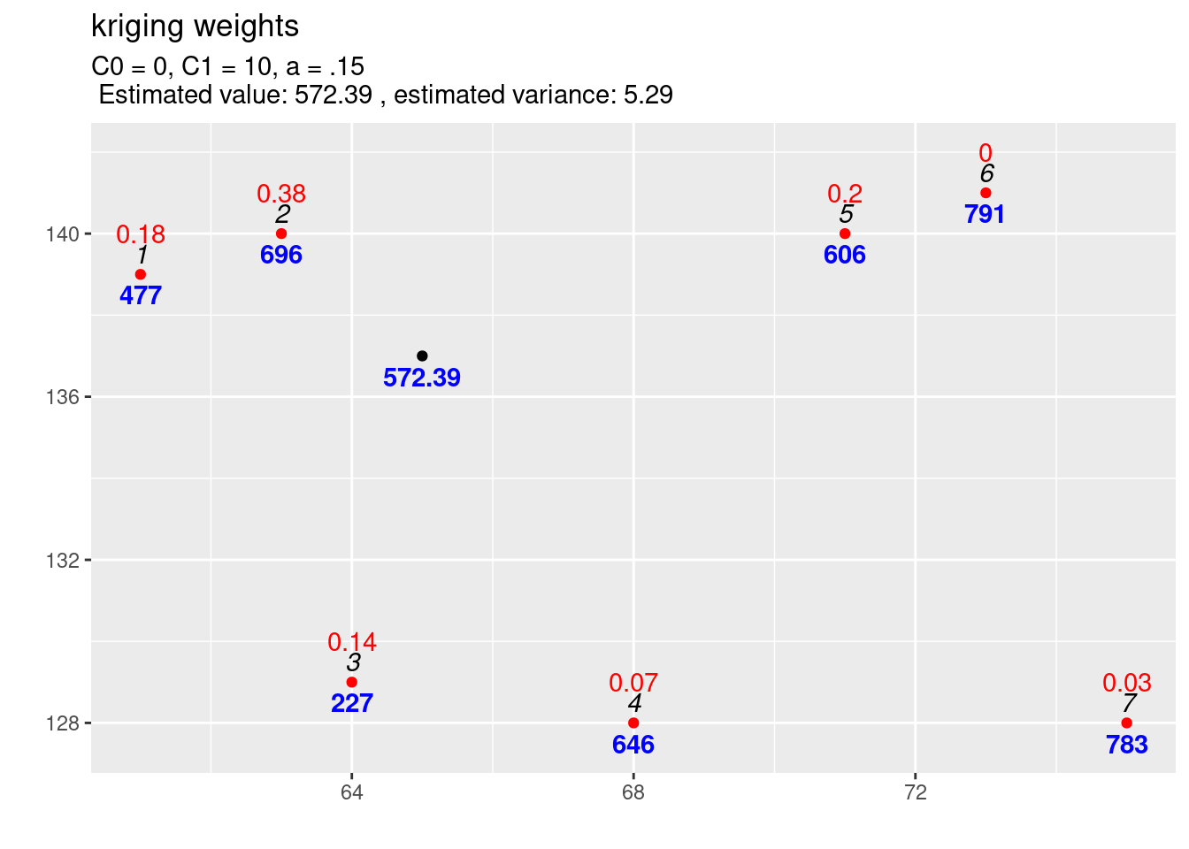
As the covariance function with the higher range increases slower it puts higher weights on closer observations and less on observations further away. This also decreased the variance of the estimation.
14.3.7.1.4 The effect of changing the variogram function
Let’s test how a different shape of the covariance function effects the kriging weights. We define a Gaussian covariance function. In contrast to the exponential covariance model we have used before, the function has a turning point. It’s second derivative is first positive and then gets negative, while the second derivative of the exponential covariance model is always negative.
gausCovFactory <- function(C0, C1, a)
{
  function(h)
    {
      res <- ifelse(h==0,
                C0 + C1,
                C1* exp(-a*h^2)  )
      return(res)
  }
}
gausCov_0_10_003 <- gausCovFactory(C0 = 0, C1 = 10, a=0.03)
ggplot() + geom_function(fun=gausCov_0_10_003) + xlim(0,20) +
geom_function(fun=expCov_0_10_03, col="blue") +
ylab("Covariance") +
xlab("Distance (h)") +
labs(title = "Covariance ",
subtitle = "For gaussian (black) and exponential (blue)")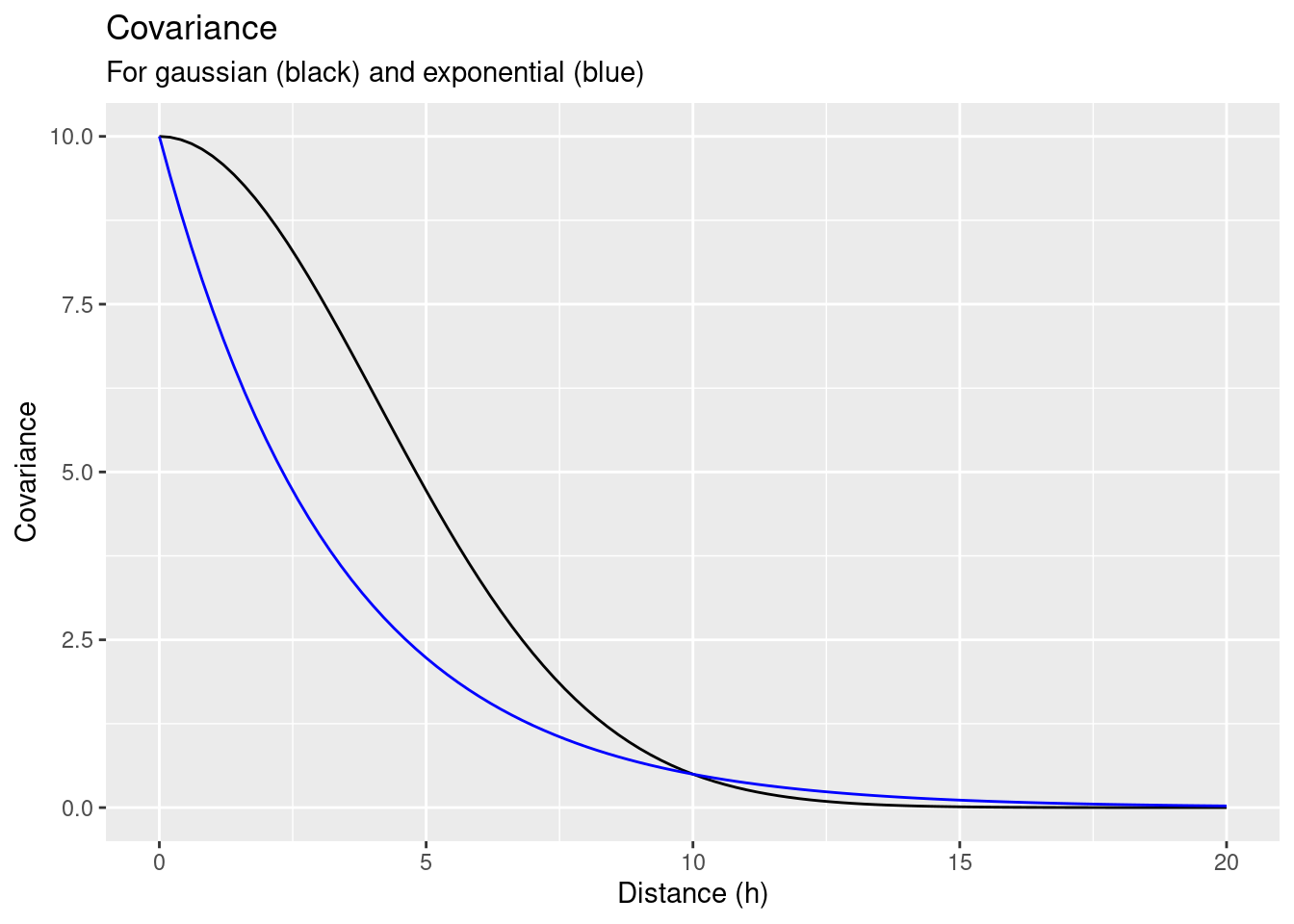
kw5 <- calcKrigingWeights(observations, newlocation, covfun = gausCov_0_10_003,
                   text4plot = "Gaussian, C0 = 0, C1 = 10, a = .03"
                  )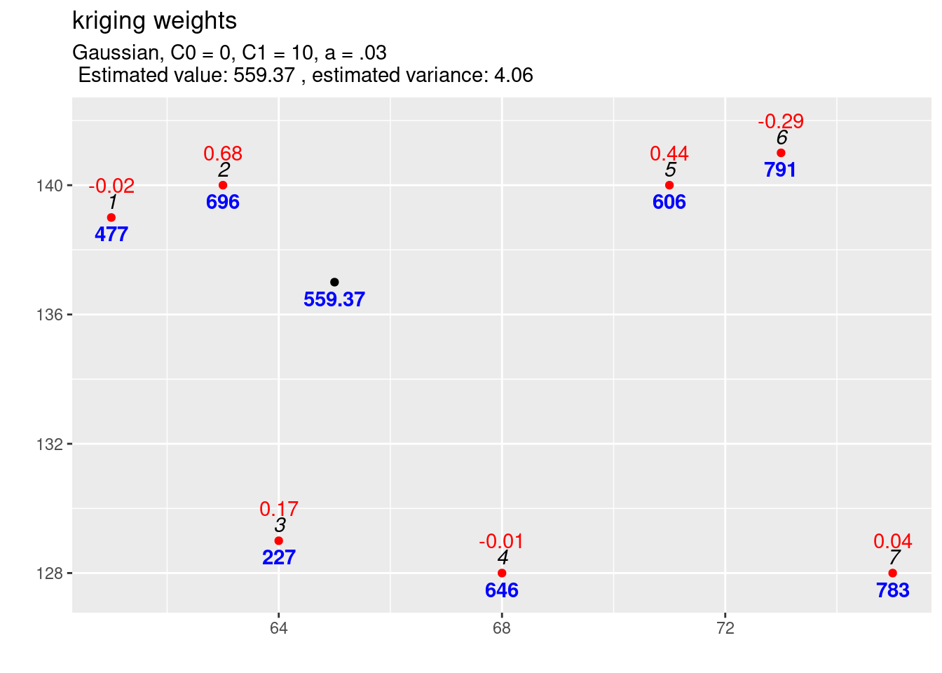
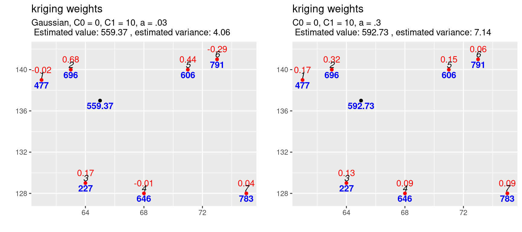
Most interesting are the negative kriging weights for observation 6, 1 and 4. The shape of the gaussian covariance model puts much more weight on the closest observation. We see that the closest observation 2 gets now 68% of the total weight. This reduces the weights of all other observations. The negative weights are the result of an effect called the screen effect. An observation is screened, if another observation is located between it and the location to be interpolated. This is what we before describe as the declustering of observations that are closely located and is caused by \(C^{-1}\). The screen effect is strong for observation 6 as observation 5 is more or less directly between the location to be interpolated and observation 6.
These types of covariance functions (or variogram functions) allow interpolation of values higher or lower than the observed values. This might be reasonable or even wanted as the sample presumably does not contain the full range of values of the underlying process \(S(x)\). However, negative weights can lead to implausible predictions, e.g. if negative concentrations or negative rainfall is predicted. These types of covariance functions might be reasonable for extremely continuous, such as the depth of a particular soil horizon. However, even for such data, these functions are often not used in practice since the negative weights tend to make the prediction very erratic (Isaaks and Srivastava, 1989, p. 305).
14.3.8 Cross-validation
Cross-validation is a commonly used way to check model performance. The basic strategy is to withhold a part of the data, fit the model with the rest of the data and assess goodness of fit for the withhold data. Often the root mean square error is used. For k-fold cross-validation, the data is split randomly in k groups. When k-1 groups are used to fit the data and the left out data is used for validation. When the next group is withhold and the goodness of fit accessed, until all groups have been withhold once. The goodness of fit indicator is summed or averaged across all k-folds. Commonly, 5-fold or 10-fold cross-validation is used. Alternatively, leave-one-out is used as a strategy - thereby, each fold consists of leaving a single observation out. As only a single point is left out, the test is often not as rigorous as for 5- or 10- fold cross-validation. If data is spatially structured, spatial cross-validation is preferable. Thereby, the data is split into k spatially connected regions instead of randomly spitting the data. At each fold, a region is left out. An easy approach is to use k-means clustering on the coordinates for the regional group assignment.
In gstat krige.cv and gstat.cv implement non-spatial cross-validation. The functions perform the cross-validation after the variogram has been fitted. If that part of the model chain should be tested as well, cross-validation needs to be implemented manually.
14.3.9 Block kriging
Geostatistics treats observations as being observed at a point location. In reality, usually the size of the observation is not zero. If one takes e.g. a soil sample this sample covers some area which might be small, but larger than zero. Using kriging for predictions at a physical size equal to that of the observations is called point kriging. In contrast, block kriging predicts averages of larger areas or volumes. The term block kriging originates from mining, where early geostatistics was developed. In mines, predictions based on bore hole data had to be made for mineable units, which tended to have a block shape. Change of support occurs when predictions are made for a larger physical support based on small physical support observations. There is no particular reason why the larger support needs to have a rectangular shape, but it is common. It is also possible to use irregularly shaped blocks, e.g. the administrative boundaries of municipalities or districts or neighborhoods if we are interested for example on the mean air temperature or mean air pollution across such a units. The ‘block’ in block kriging therefore has to be interpreted as ‘a spatially connected area for which we would like to obtain an average predicted value’, not necessarily a rectangular unit.
A nice property of block kriging is that by averaging the prediction much of the variability averages out, leading to lower prediction errors for block averages. The averaging is of course stronger for larger areas. If blocks are getting too big, we lose of course spatial patter. So we often try to use blocks that are big enough to substantially reduce the prediction errors but small enough to reveal spatial pattern. In environmental problems, legislation may be related to means or medians over larger areas, rather than to point values.
Block kriging (or other forms of prediction for blocks) can be obtained by gstat in three ways:
- For regular blocks, by specifying a block size
- For irregular but constant ‘blocks’, by specifying points that discretize the irregular form
- For blocks or areas of varying size, by passing an object of class SpatialPolygons to the newdata argument
For block kriging our \(C\) covariance matrix is unchanged, only the covariance matrix for the new location \(c_0\) changes:
\[ \left[\begin{array} {c} w_1(s_0)\\ \vdots \\ w_n(s_0)\\ \xi \end{array}\right] = \left[\begin{array} {cccc} C(s_1,s_1) & \ldots & C(s_1,s_n) & 1 \\ \vdots & \vdots & \vdots & \vdots \\ C(s_n,s_1) & \ldots & C(s_n,s_n) & 1 \\ 1 & \ldots & 1 & 0 \end{array}\right]^{-1} \cdot \left[\begin{array} {c} \bar{C}(s_A,s_1)\\ \vdots \\ \bar{C}(s_A,s_n)\\ 1 \end{array}\right] \]
where \(\bar{C}(s_A, s_i)\) is the average covariance between a particular observation \(i\) and all of the points between the area \(A\):
\[\bar{C}(s_A, s_i) = \frac{1}{|A|} \sum_{j| j \epsilon A}C_{ij}\]
The block kriging variance is given by:
\[ \hat{sigma}^2_{ok} = \bar{C}(s_A, s_A)-(\sum_{i=1}^nw_i\bar{C}(s_A, s_i) + \mu) \]
\(\bar{C}(s_A, s_A)\) is the average covariance between pairs of locations within the area \(A\):
\[ \bar{C}(s_A, s_A) = \frac{1}{|A|^2} \sum_{i|i\epsilon A} \sum_{j|j\epsilon A} C(s_i, s_j)\]
In practice, the block kriging covariance is estimated by discretizing the area \(A\) into several points. The same discretization needs to be used for the point to block covariance \(c_0\) and for the block kriging variance.
14.3.10 Local kriging
So far, we have always used all data points for the interpolation. It is also possible, to use local kriging that used only a neighborhood around the location to be estimated, e.g. by defining a search distance and/or a minimal number of nearest neighbors that should be used. One reason for doing so is computational efficiency, as estimations can be significantly faster if only a subset of the full dataset is used. However, if the subset is chosen too big, computation tim might even increase. The reason for that is, that for global kriging \(C\) has to be inverted only once while for local kriging \(C\) differs for each location - therefore each time a different \(C\) matrix has to be inverted which is time consuming. Another motivation for local kriging is statistical: if we have reason to believe that the mean is not stationary over the whole area but only for smaller parts of the area, this can be modeled by local kriging.
14.3.11 Cokriging
Cokriging uses cross-correlation between several variables to minimize the variance of the estimation error. This works of course only, if the correlation between the two measured variables is strong enough. Cokriging is especially useful, when the primary variable of interest is hard or costly to measure and therefore undersampled, while the secondary variable is easier or cheaper to measure. If soil organic matter is easier to measure than heavy meal concentration in the top soil and if organic matter is a god proxy for the heavy metal concentration, cokriging might be the way to go.
The prediction for the primary variable \(\hat{u}_0\) is based again on the observed values for \(u\) and the kriging weights obtained via the semivariogram. However, the equation considers the observed secondary values \(v\) as well:
\[ \hat{u}_0 = \sum_{i=1}^{n}a_i u_i + \sum_{j=1}^{m}b_j v_j \] where \(a_i\) and \(b_j\) are cokriging weights.
The estimation error is expressed similar to ordinary kriging by:
\[ R = \hat{u}_0 - u_0 = \sum_{i=1}^{n}a_i u_i + \sum_{j=1}^{m}b_j v_j -u_0 ´\] The minimzed variance of the estimation error can be calculated by:
\[ var(R) = cov(u_0, u_0) + \mu_1 - \sum_{i=1}^n a_i \cdot cov(u_i, u_0) - \sum_{j=1}^{m}b_j \cdot cov(v_j, u_0)\]
where \(\mu_1\) is a Lagrange multiplier. (Cokriging can be easily extended to more auxillary variables.)
The auto- and cross-variogram must thereby be constructed the same basis variogram model.
14.3.12 Further reading
An excellent and accessible (given a mathy topic as kriging) is (Isaaks and Srivastava, 1989). Their book focuses on ordinary kriging.
A more mathy approach is followed by (Diggle and Ribeiro, 2007), who use the geoR package for demonstrations. They cover quite some ground and highlight applications beyond interpolation.
Somewhere inbetween is the work by (Hengl et al., 2007) who use gstat as well as geoR and standard GIS software such as SAGA for their demonstrations.
14.4 Case study: Interpolation of temperature data in Germany
We will use kriging to interpolate temperature data in Germany. You might recall the example from the Einführung in die Geoinformatik as I used the same data to demonstrate some basic interpolation techniques such as IDW, thiess polygons or natural neighbors. The climate data is historic ~1940-1980.
The data consistst of a shapefile that contains the location of temperature stations together with some information about the station (such as the name, the elevation). An external file consists the long time average temperature data and can be joined to the station data based on a common attribute file. As temperature clearly depends on elevation we will also use a digital elevation model in a raster format.
14.4.1 Data pre-processing
14.4.1.1 Temperature stations
To read the data as an sf object we use st_read. The dsn equals for a shapefile the path to the folder (remember to use the slash and not the backslash if you are working on a MS Windows machine), the name of the layer is the name of the shapefile without the file extension.
## Reading layer `temp_stations' from data source
##   `/home/slautenbach/Documents/lehre/HD/git_areas/spatial_data_science/spatial-data-science/data'
##   using driver `ESRI Shapefile'
## Simple feature collection with 285 features and 13 fields
## Geometry type: POINT
## Dimension:     XY
## Bounding box:  xmin: 4.93 ymin: 45.03 xmax: 16.88 ymax: 56.8
## Geodetic CRS: WGS 84## AREA PERIMETER TEMP_STATI TEMP_STA_1 COUNTRY_ID
## Min. :0 Min. :0 Min. :4856 Min. : 260600 Min. :602.0
## 1st Qu.:0 1st Qu.:0 1st Qu.:5123 1st Qu.: 678200 1st Qu.:612.0
## Median :0 Median :0 Median :5327 Median :1031700 Median :618.0
## Mean :0 Mean :0 Mean :5293 Mean : 964310 Mean :616.5
## 3rd Qu.:0 3rd Qu.:0 3rd Qu.:5398 3rd Qu.:1103600 3rd Qu.:619.0
## Max. :0 Max. :0 Max. :5630 Max. :1611000 Max. :627.0
## NAME LAT LON ELEV
## Length:285 Min. :45.03 Min. : 4.93 Min. :-999.0
## Class :character 1st Qu.:47.42 1st Qu.: 8.40 1st Qu.: 56.0
## Mode :character Median :50.03 Median :10.62 Median : 238.0
## Mean :50.08 Mean :10.77 Mean : 409.8
## 3rd Qu.:52.25 3rd Qu.:13.40 3rd Qu.: 474.0
## Max. :56.80 Max. :16.88 Max. :3580.0
## FIRST LAST MISSING DISC geometry
## Min. :1701 Min. :1920 Min. : 0.000 Min. :0 POINT :285
## 1st Qu.:1953 1st Qu.:1990 1st Qu.: 1.700 1st Qu.:0 epsg:4326 : 0
## Median :1981 Median :1990 Median : 1.700 Median :0 +proj=long...: 0
## Mean :1953 Mean :1988 Mean : 5.659 Mean :0
## 3rd Qu.:1981 3rd Qu.:1990 3rd Qu.: 4.200 3rd Qu.:0
## Max. :1981 Max. :1990 Max. :68.900 Max. :0The interesting fields are as follows: - ELVE - elevation above mean sea level in meter - FIRST - year of the first recording - LAST - year of the last recording - MISSING - percentage of missing data - TEMP_STA_1 - the ID, used to link the external data to the stations
14.4.1.1.1 Do we need to filter the data
We might want to exclude stations at which measurements ended to early or for which the time series used to calculate the average are to short. In addition we want to exclude those there elevation is missing (-999).
Eleven stations have stopped recording before 1970. A few even before the end of world war II.
## Simple feature collection with 11 features and 13 fields
## Geometry type: POINT
## Dimension:     XY
## Bounding box:  xmin: 8.3 ymin: 46.5 xmax: 15 ymax: 56.8
## Geodetic CRS:  WGS 84
## First 10 features:
##    AREA PERIMETER TEMP_STATI TEMP_STA_1 COUNTRY_ID             NAME   LAT   LON
## 1     0         0       5049     605201        608        VESTERVIG 56.80  8.30
## 2     0         0       5050     605801        608             TARM 55.90  8.50
## 3     0         0       5059     615001        608             BOGO 54.90 12.10
## 4     0         0       5278     917700        618          TETEROW 53.77 12.62
## 5     0         0       5298     946902        618          LEIPZIG 51.40 12.40
## 6     0         0       5307     955401        618           WEIMAR 51.00 11.30
## 7     0         0       5328    1032000        618       GUETERSLOH 51.92  8.30
## 8     0         0       5355    1064002        618 FRANKFURT A MAIN 50.10  8.70
## 9     0         0       5414    1123101        619             OBIR 46.50 14.50
## 10    0         0       5417    1141800        620  MARIANSKE LAZNE 49.92 12.72
##    ELEV FIRST LAST MISSING DISC            geometry
## 1    19  1874 1969     3.1    0    POINT (8.3 56.8)
## 2     7  1861 1969     3.7    0    POINT (8.5 55.9)
## 3    27  1873 1969     3.4    0   POINT (12.1 54.9)
## 4    46  1951 1960     0.0    0 POINT (12.62 53.77)
## 5   137  1759 1935    29.1    0   POINT (12.4 51.4)
## 6   268  1951 1960     0.0    0     POINT (11.3 51)
## 7    72  1835 1920     0.0    0   POINT (8.3 51.92)
## 8   109  1757 1961    19.9    0    POINT (8.7 50.1)
## 9  2044  1851 1944     0.5    0   POINT (14.5 46.5)
## 10  541  1951 1960     0.0    0 POINT (12.72 49.92)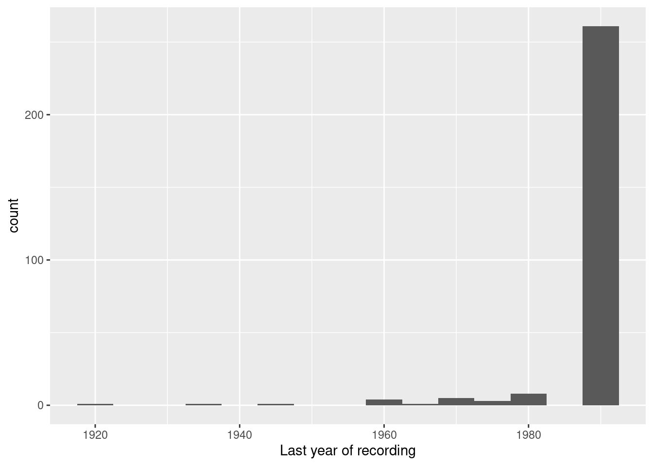
## Simple feature collection with 3 features and 13 fields
## Geometry type: POINT
## Dimension:     XY
## Bounding box:  xmin: 6.02 ymin: 49.8 xmax: 12.82 ymax: 55.38
## Geodetic CRS:  WGS 84
##   AREA PERIMETER TEMP_STATI TEMP_STA_1 COUNTRY_ID       NAME   LAT   LON ELEV
## 1    0         0       4858     261600        602  FALSTERBO 55.38 12.82 -999
## 2    0         0       5097     658500        611   CLERVAUX 50.05  6.02 -999
## 3    0         0       5099     659700        611 ECHTERNACH 49.80  6.45 -999
##   FIRST LAST MISSING DISC            geometry
## 1  1981 1990     1.7    0 POINT (12.82 55.38)
## 2  1971 1980     0.0    0  POINT (6.02 50.05)
## 3  1971 1980     4.2    0   POINT (6.45 49.8)
How long are the time series used to calculate the average?
stations %>% mutate(duration = LAST - FIRST) %>%
  ggplot(aes(x=duration)) + geom_histogram(binwidth = 5) +
  xlab("Length of recording period [years]")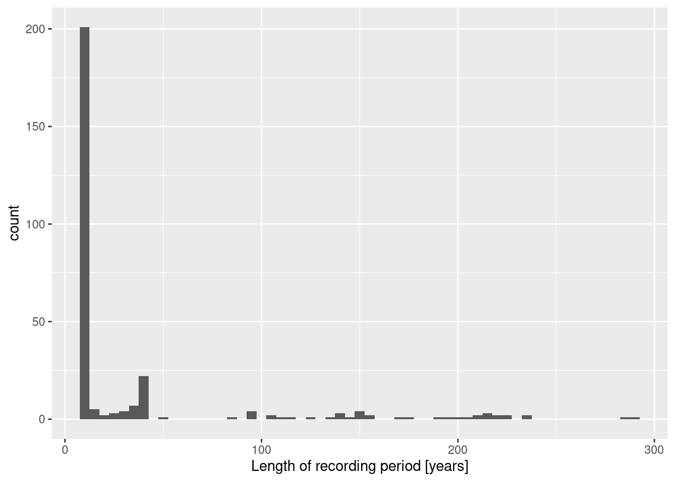
As we, the majority of stations had a recording period of less than 10 years. All stations have a recording period of at least 9 years.
## Simple feature collection with 0 features and 13 fields
## Bounding box:  xmin: NA ymin: NA xmax: NA ymax: NA
## Geodetic CRS:  WGS 84
##  [1] AREA       PERIMETER  TEMP_STATI TEMP_STA_1 COUNTRY_ID NAME
##  [7] LAT        LON        ELEV       FIRST      LAST       MISSING
## [13] DISC       geometry
## <0 rows> (or 0-length row.names)
stations %>% mutate(duration = LAST - FIRST) %>%
ggplot(aes(x=FIRST, y=duration)) + geom_point(alpha=.5) +
xlab("Year of first recording") + ylab("Length of recording period [years]")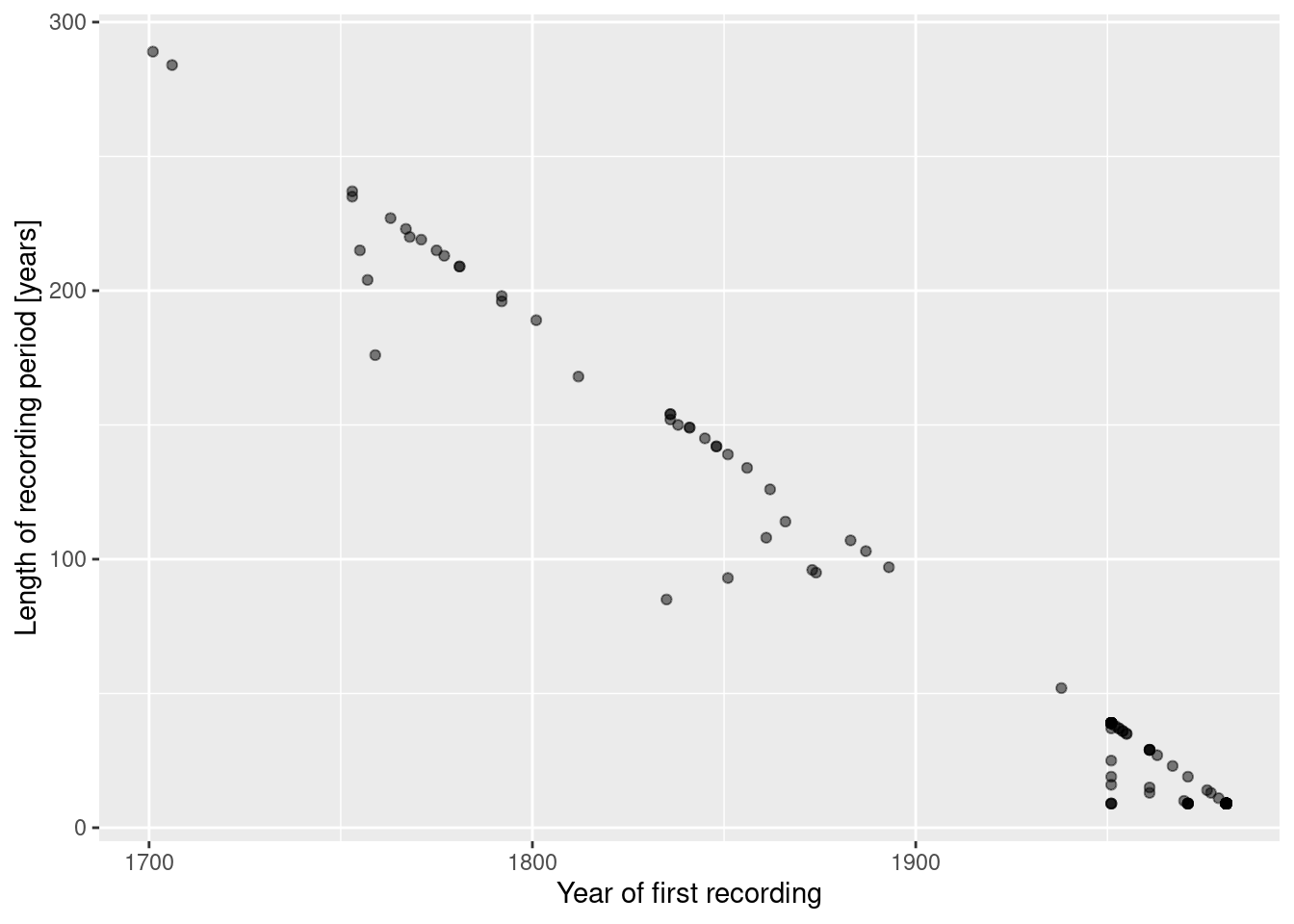
Not unexpectedly, newer stations have a shorter period of recording.
What about the missing data?
stations %>% mutate(duration = LAST - FIRST) %>%
  ggplot(aes(x=FIRST, y=MISSING, color = duration)) + geom_point(alpha=.5) +
  xlab("Year of first recording") + ylab("Missing data [%]") +
scale_color_continuous(name = "Duration of recording") 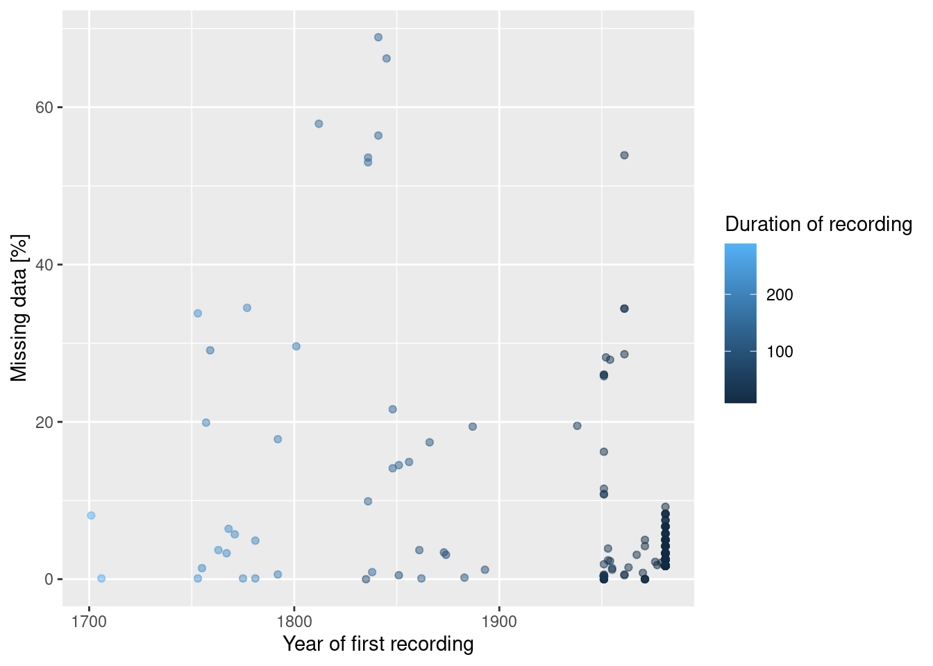
The stations with large shares of missing also have long recording periods. Therefor, we might want to keep them.
Now it is time to make a decisions. Which stations do we want to keep, which ones do we want to drop?
The answer depends on the purpose of the analysis. The trade-off is between comparability of the different stations and the density of stations available. I would tend to keep as many stations as possible for our interpolation but to check if largest errors occur for stations with short recording periods, many missing observations or which stopped recording a while ago. We might as well compare our results against the interpolation we get based on a stricter selection. After all, this is just a classroom example and not a real world analysis for which we would pay much more attention to such issues.
Let’s keep everything but drop the stations with missing information about elevation.
14.4.1.2 Temperature data
The data is stored in a dbase IV file which we can load with read.dbf, a function from the foreign package.
##    STATION_ID           JAN               FEB               MAR
##  Min.   : 100100   Min.   :-47.705   Min.   :-44.330   Min.   :-57.9570
##  1st Qu.:3171600   1st Qu.: -6.146   1st Qu.: -4.769   1st Qu.: -0.1325
##  Median :6450000   Median :  1.733   Median :  3.043   Median :  6.4890
##  Mean   :5460681   Mean   :  3.205   Mean   :  4.479   Mean   :  7.9566
##  3rd Qu.:7257246   3rd Qu.: 15.015   3rd Qu.: 15.934   3rd Qu.: 17.9535
##  Max.   :9909001   Max.   : 32.678   Max.   : 31.589   Max.   : 32.3880
##       APR               MAI              JUN              JUL
##  Min.   :-64.757   Min.   :-65.64   Min.   :-65.25   Min.   :-66.92
##  1st Qu.:  6.069   1st Qu.: 11.34   1st Qu.: 14.95   1st Qu.: 17.25
##  Median : 11.262   Median : 15.67   Median : 19.21   Median : 21.58
##  Mean   : 12.231   Mean   : 16.12   Mean   : 19.12   Mean   : 20.91
##  3rd Qu.: 19.116   3rd Qu.: 21.57   3rd Qu.: 24.40   3rd Qu.: 25.79
##  Max.   : 34.123   Max.   : 35.76   Max.   : 36.94   Max.   : 38.30
##       AUG              SEP              OCT               NOV
##  Min.   :-67.66   Min.   :-66.01   Min.   :-57.172   Min.   :-43.3720
##  1st Qu.: 16.45   1st Qu.: 12.85   1st Qu.:  7.867   1st Qu.:  0.9895
##  Median : 20.90   Median : 17.53   Median : 12.570   Median :  6.8670
##  Mean   : 20.40   Mean   : 17.56   Mean   : 13.451   Mean   :  8.3392
##  3rd Qu.: 25.57   3rd Qu.: 23.48   3rd Qu.: 20.489   3rd Qu.: 17.9685
##  Max.   : 37.01   Max.   : 34.79   Max.   : 32.470   Max.   : 33.2450
##       DEC               YEAR
##  Min.   :-45.784   Min.   :-55.280
##  1st Qu.: -3.975   1st Qu.:  6.478
##  Median :  3.258   Median : 11.505
##  Mean   :  4.605   Mean   : 12.365
##  3rd Qu.: 15.650   3rd Qu.: 19.316
##  Max.   : 32.855   Max.   : 31.108
STATION_ID is the station ID, the other colums contain the yearly or monthly temperature means.
Let’s join the data to the stations. The only thing we need to specify are the field names.
Get an OSM background map.
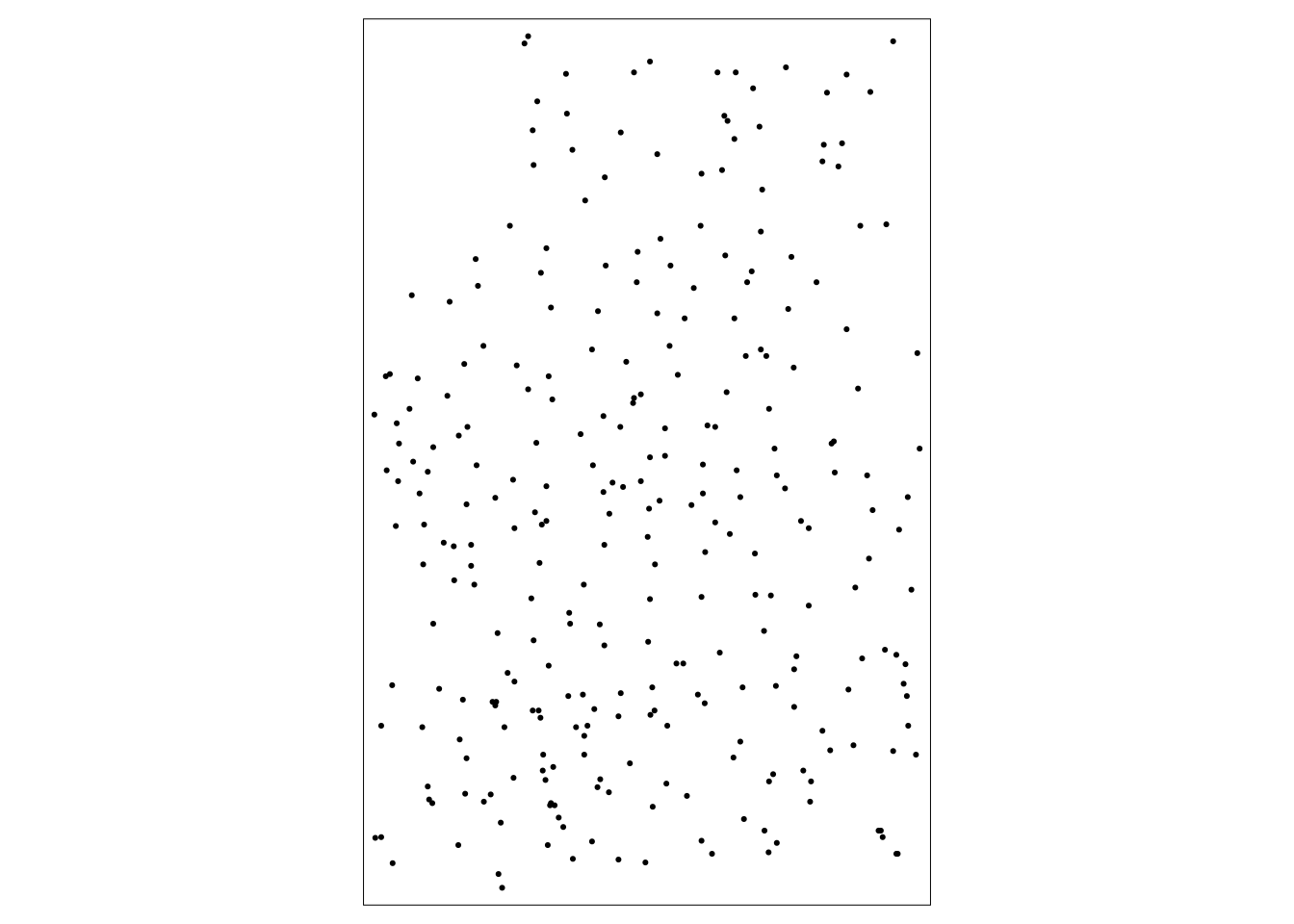
tm_shape(osmbg) + tm_rgb() +
tm_shape(tempStations) + tm_dots(col="YEAR", size=.2, title ="Temperature [°C]", midpoint=0) +
  tm_scale_bar() +
  tm_layout(attr.outside = TRUE, legend.outside = TRUE, main.title = "Long term yearly average temperature")
## ## ── tmap v3 code detected ───────────────────────────────────────────────────────## [v3->v4] `tm_tm_dots()`: migrate the argument(s) related to the scale of the
## visual variable `fill` namely 'midpoint' to fill.scale = tm_scale(<HERE>).
## ℹ For small multiples, specify a 'tm_scale_' for each multiple, and put them in
## a list: 'fill.scale = list(<scale1>, <scale2>, ...)'
## [v3->v4] `tm_dots()`: use 'fill' for the fill color of polygons/symbols
## (instead of 'col'), and 'col' for the outlines (instead of 'border.col').
## [tm_dots()] Argument `title` unknown.
## ! `tm_scale_bar()` is deprecated. Please use `tm_scalebar()` instead.
## [v3->v4] `tm_layout()`: use `tm_title()` instead of `tm_layout(main.title = )`
## [plot mode] fit legend/component: Some legend items or map compoments do not
## fit well, and are therefore rescaled.
## ℹ Set the tmap option `component.autoscale = FALSE` to disable rescaling.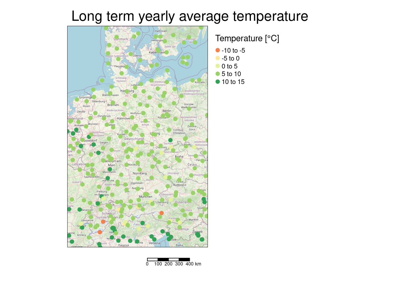
The few “cold spots” are presumably located in the Alps and therefore heavily affected by the terrain.
Before the interpolation it is essential to transform the stations data to a metric coordinate system. Geographic coordinates are in general not well suited. However, more and more spatial functions in R are capable of working properly with geographic coordinate systems.
Let’s also store the transformed x and y coordinates as columns - we need them later on.
14.4.1.3 Elevation raster
## class       : SpatRaster
## dimensions  : 1541, 1864, 1  (nrow, ncol, nlyr)
## resolution  : 0.00833333, 0.00833333  (x, y)
## extent      : 2.088879, 17.62221, 44.53262, 57.37428  (xmin, xmax, ymin, ymax)
## coord. ref. : lon/lat WGS 84 (EPSG:4326)
## source      : dem.tif
## name        :  dem
## min value   :   -4
## max value   : 3855
Set maximum raster cells to avoid downsampling
tm_shape(elev) +
  tm_raster(col="dem",
            col.scale= tm_scale_intervals(values = "brewer.greys", style= "fixed", breaks = c(-15, 0, 100, 250, 500, 1000, 4300), midpoint= NA),
            col.legend= tm_legend(title= "Elevation [m]")) +
  tm_shape(tempStations) +
  tm_dots(col="YEAR", col.scale= tm_scale_intervals(midpoint=NA),
          col.legend= tm_legend(title ="Temperature [°C]"),
          size.scale= tm_scale(size=.2) ) +
  tm_scalebar() +
  tm_layout(attr.outside = TRUE, legend.outside = TRUE ) +
  tm_title("Long term yearly average temperature")
## [plot mode] fit legend/component: Some legend items or map compoments do not
## fit well, and are therefore rescaled.
## ℹ Set the tmap option `component.autoscale = FALSE` to disable rescaling.
We also need to transform the raster to the same coordinate system as the station data.
14.4.2 Explorative data analysis
We want to check for the effect of co-variates (elevation) and for a spatial trend in the data.
We will do this by< means of a linear model that uses elevation and latitude and longitude as predictors for the long term average yearly temperature.
##
## Call:
## lm(formula = YEAR ~ ELEV + LAT + LON, data = tempStations)
##
## Residuals:
## Min 1Q Median 3Q Max
## -1.65811 -0.35264 -0.07791 0.29900 2.13109
##
## Coefficients:
## Estimate Std. Error t value Pr(>|t|)
## (Intercept) 3.432e+01 6.914e-01 49.635 < 2e-16 ***
## ELEV -5.240e-03 7.046e-05 -74.366 < 2e-16 ***
## LAT -4.565e-01 1.348e-02 -33.872 < 2e-16 ***
## LON -9.256e-02 1.163e-02 -7.956 4.53e-14 ***
## ---
## Signif. codes: 0 '***' 0.001 '**' 0.01 '*' 0.05 '.' 0.1 ' ' 1
##
## Residual standard error: 0.6247 on 278 degrees of freedom
## Multiple R-squared: 0.9526, Adjusted R-squared: 0.9521
## F-statistic: 1864 on 3 and 278 DF, p-value: < 2.2e-16Clearly all three predictors have a significant effect. Temperature is dropping by 0.524°C per 100m elevation, by 0.457°C for each degree we move northwards and by 0.09°C for each degree we move to the east.
ggplot(tempStations, aes(x=ELEV, y=YEAR, color=LAT)) +
geom_point() +
geom_smooth(method="lm") +
xlab("Elevation [m]") + ylab("Yearly average temperature [°C]")## `geom_smooth()` using formula = 'y ~ x'## Warning: The following aesthetics were dropped during statistical transformation:
## colour.
## ℹ This can happen when ggplot fails to infer the correct grouping structure in
## the data.
## ℹ Did you forget to specify a `group` aesthetic or to convert a numerical
## variable into a factor?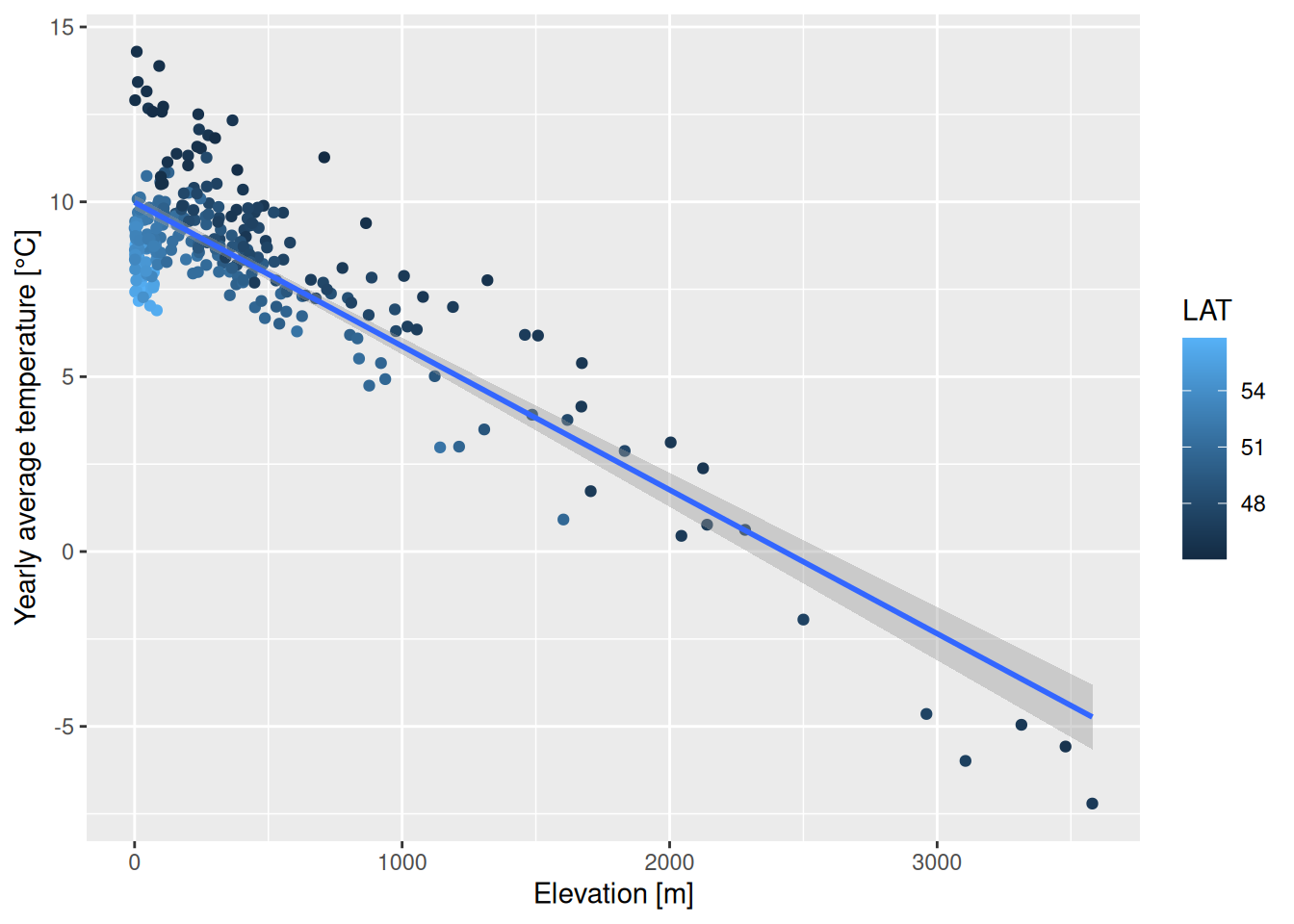
This violates the assumption of stationarity. Therefore, we need to correct this effect. We could either do this in the attribute table of the station sf object or let gstat take care of that for us. If we specify a regression formula gstat uses external drift kriging aka regression kriging. The benefit of the later approach is that this includes the uncertainty by the regression kriging aka universal kriging. For pedagogical reasons we will explore and compare both approaches.
We might as well use the transformed coordinates - which is preferable as distances based on geographic coordinates differ in space.
##
## Call:
## lm(formula = YEAR ~ ELEV + X + Y, data = tempStations)
##
## Residuals:
## Min 1Q Median 3Q Max
## -1.64172 -0.34835 -0.07576 0.29464 2.13071
##
## Coefficients:
## Estimate Std. Error t value Pr(>|t|)
## (Intercept) 1.008e+01 4.551e-02 221.600 < 2e-16 ***
## ELEV -5.255e-03 6.993e-05 -75.148 < 2e-16 ***
## X -1.267e-06 1.599e-07 -7.924 5.59e-14 ***
## Y -4.142e-06 1.204e-07 -34.418 < 2e-16 ***
## ---
## Signif. codes: 0 '***' 0.001 '**' 0.01 '*' 0.05 '.' 0.1 ' ' 1
##
## Residual standard error: 0.6189 on 278 degrees of freedom
## Multiple R-squared: 0.9535, Adjusted R-squared: 0.953
## F-statistic: 1901 on 3 and 278 DF, p-value: < 2.2e-1614.4.3 Manual removal of spatial trend and effect of elevation
We can directly extract the regression coefficients for use in the formula to remove the trend and the effect of elevation.
## (Intercept) ELEV X Y
## 1.008443e+01 -5.254877e-03 -1.266705e-06 -4.142351e-06tempStations <- tempStations %>%
mutate(yearNoTrend = YEAR - ELEV*coef(g)[2] - X * coef(g)[3] - Y * coef(g)[4])ggplot(tempStations, aes(x=YEAR, y= yearNoTrend)) +
geom_point(alpha=0.5) +
xlab("Original temperature [°C]") +
ylab("Detrended temperature [°C]")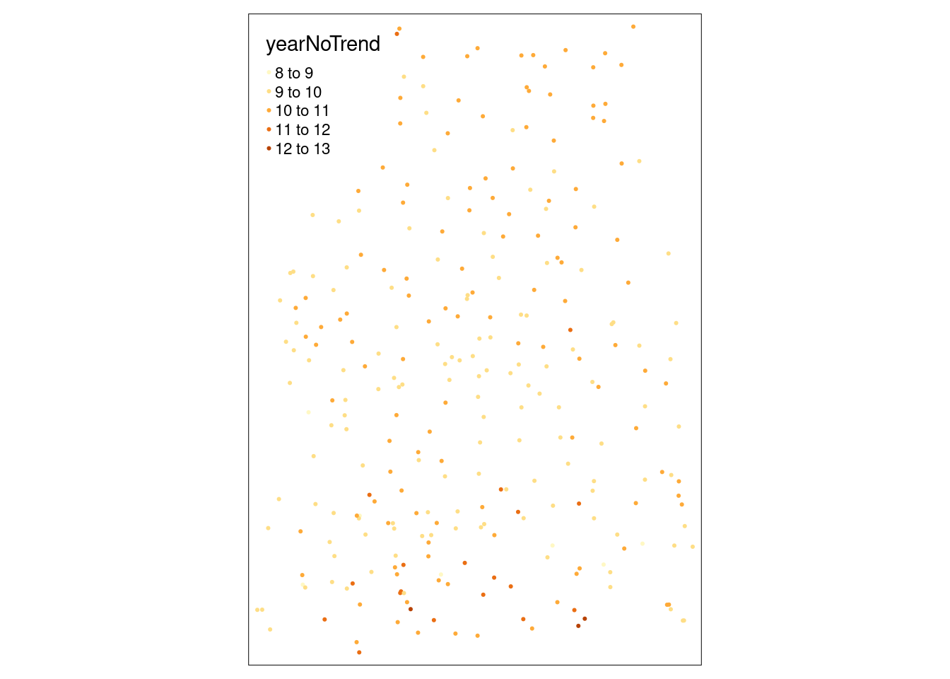
We see that at some location (south of the Alps) that stations in short distance differ in value. This might be a reason for relatively strong variability of station pairs at short distance.
14.4.3.1 Ordinary kriging of detrended yearly temperature
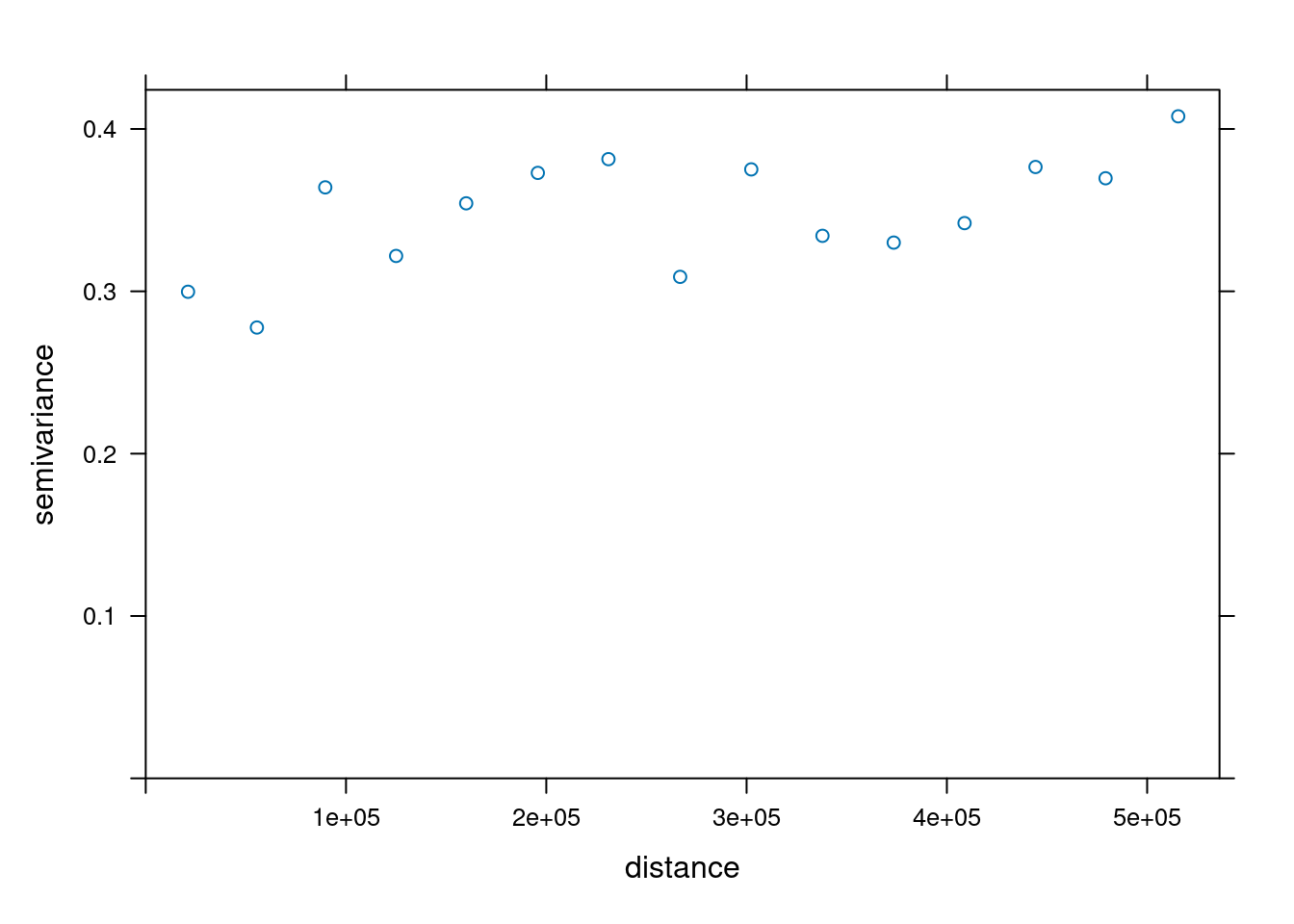
To understand how the semivariance changes with distance we plot the variogram for the detrended temperature data.
The semivariance describes the variance of the difference between observations inside a distance interval. What we expect is an increase of the semivariance with distance that levels of at a specific distance.

The semivariogram is relatively flat, indicating that the difference between observations does not differ very strongly after we removed the effect of elevation and the spatial trend. We also see a large nugget effect - for small distances we see a relatively large variability. This indicates that temperatures at station relatively close to each other are variable.
Next, we fit a theoretical variogram to the data. As we have seen, we need to include a nugget effect. The function fit.variogram is used to fit a model. It takes the empirical variogram as an input together with a specification of the model, specified by vgm. Here we use the Sperical model which allows easier interpretation of the parameters. We need to specify that we want to include a nugget effect by providing an initial value (to be estimated from the empirical variogram above).
tempNoTrend.vgm <- fit.variogram(tempNoTrend.svar, model=vgm(model="Sph", nugget = 0.1),
fit.ranges=TRUE)
tempNoTrend.vgm## model psill range
## 1 Nug 0.28072120 0.0
## 2 Sph 0.07741156 218941.3The parameter estimates tell us that a semivariance of 0.28 is estimated for pairs at a distance of 0m. The sill (the additional semivariance added to the nugget effect) has been estimated as 0.08. This effect is relatively week compared to the nugged effect. The theoretical variogram levels of at a distance of 218.94 km.
We can also plot the fitted theoretical variogram to get a better impression:
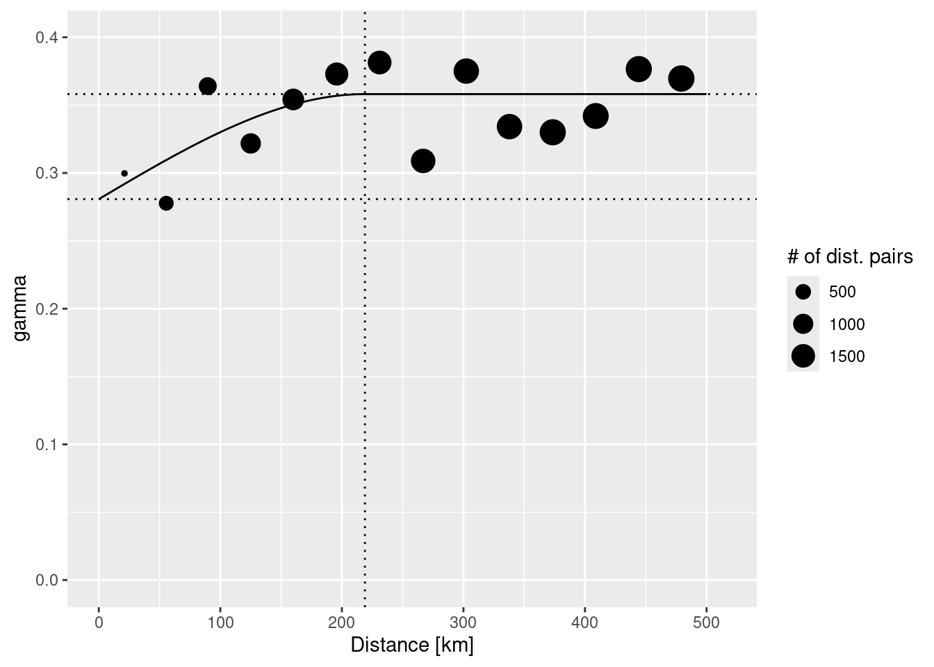
The plot command for variogram objects is a bit limited. Therefore, we use ggplot2 to create a plot with added lines for the different model components. In addition we use the size of the dots to represent the number of distance pairs in each bin. tempNoTrend.svar is a data frame with the necessary components: np - number of distance pairs, dist - distance class, gamma - the semivariance. To add the fitted theoretical variogram we use variogramLine which predicts values for the variogram model we supply.
vgmPrediction <- variogramLine(tempNoTrend.vgm, maxdist= 5*10^5)
ggplot(tempNoTrend.svar,aes(x=dist / 1000,y=gamma,size=np)) + geom_point() +
geom_line(data= vgmPrediction, mapping=aes(x=dist/1000,y=gamma), inherit.aes = FALSE) +
geom_hline(yintercept = tempNoTrend.vgm$psill[1], lty=3) +
geom_hline(yintercept = sum(tempNoTrend.vgm$psill), lty=3) +
geom_vline(xintercept = tempNoTrend.vgm$range[2]/1000, lty=3) +
ylim(0, 0.4) + scale_size_continuous(name="# of dist. pairs") +
xlab("Distance [km]")## Warning: Removed 1 row containing missing values or values outside the scale range
## (`geom_point()`).
We need to specify a point sf or sp layer for the interpolation. We take the elevation raster as a template. Unfortunatley, we can currently not use a raster layer directly. We convert the raster to an sp point layer. As it has a regular structure we set the gridded attribute which makes it easier to convert the result to a raster afterwards. As we need x and y coordinates for the backtransformation (retrending the result) we store x ad y coordinates in the spGriddedPointDataFrame. The conversion by rasterToPoints ignores all cells with no-data information - i.e. the sea areas are excluded.
#predLocations <- rasterToPoints(elev, spatial = TRUE )
predLocations <- as.points(elev )
predLocations <- as(predLocations, "Spatial")
#predLocations$X <- coordinates(predLocations)[,1]
#predLocations$Y <- coordinates(predLocations)[,2]
gridded(predLocations) <- TRUENow we perform ordinary kringing (no trend). We need to specify the formula, the locations with the point data used for the interpolation (we need to convert them to a sp object). Furthermore, we need to specify the model to be used (the fitted theoretical variogram) and the locations for which we would like to get the predictions for (newdata).
The result is then converted to a raster brick (raster with several layers) which contains the prediction and the standard error of the prediction.
tempStations_sp <- as(tempStations, "Spatial")
crs(tempStations_sp) <- crs(predLocations) # ensure CRS is exactly the same
# see https://stackoverflow.com/questions/32379537/adding-crs-in-sp-seems-inconsistent
predTempNoTrend <- krige(yearNoTrend ~ 1, locations = tempStations_sp, newdata = predLocations, model = tempNoTrend.vgm)## [using ordinary kriging]Alternative variant using raster:
xxx <- raster(elev) # convert terra object to raster
gOK <- gstat(NULL, "tempDetrended", yearNoTrend ~ 1, tempStations_sp, model=tempNoTrend.vgm)
OK <- interpolate(xxx, gOK)## [using ordinary kriging]## [using ordinary kriging]To get the standard errors we need to call interpolate a second time with a different function (predict.se).
If we check results we set that - beside a different extent as no-data cells are treated differently - results are exactly the same (as it should be).
## Warning in OK - subset(predTempNoTrendRas, "var1.pred"): Raster objects have
## different extents. Result for their intersection is returned## class : RasterLayer
## dimensions : 1354, 950, 1286300 (nrow, ncol, ncell)
## resolution : 1000, 1000 (x, y)
## extent : -435780.9, 514219.1, -668254, 685746 (xmin, xmax, ymin, ymax)
## crs : +proj=lcc +lat_0=51 +lon_0=10.5 +lat_1=48.6666666666667 +lat_2=53.6666666666667 +x_0=0 +y_0=0 +ellps=GRS80 +towgs84=0,0,0,0,0,0,0 +units=m +no_defs
## source : memory
## names : layer
## values : 0, 0 (min, max)## Warning in OK.se - -subset(predTempNoTrendRas, "var1.var"): Raster objects have
## different extents. Result for their intersection is returned## class : RasterLayer
## dimensions : 1354, 950, 1286300 (nrow, ncol, ncell)
## resolution : 1000, 1000 (x, y)
## extent : -435780.9, 514219.1, -668254, 685746 (xmin, xmax, ymin, ymax)
## crs : +proj=lcc +lat_0=51 +lon_0=10.5 +lat_1=48.6666666666667 +lat_2=53.6666666666667 +x_0=0 +y_0=0 +ellps=GRS80 +towgs84=0,0,0,0,0,0,0 +units=m +no_defs
## source : memory
## names : layer
## values : 10.04729, 11.21365 (min, max)Let’s see what we have got.
## ℹ tmap mode set to "plot".tm_shape(predTempNoTrendRas %>% subset(subset="var1.pred")) +
tm_raster(col="var1.pred", title = "Prediction [°C]") +
tm_shape(tempStations) +
tm_dots(col="yearNoTrend", title = "Observed [°C]", palette = "Reds") +
tm_scale_bar() +
tm_layout(title = "Detrended temperature interpolation, ok",
legend.outside = TRUE, attr.outside = TRUE)##
## ── tmap v3 code detected ───────────────────────────────────────────────────────
## [v3->v4] `tm_raster()`: migrate the argument(s) related to the legend of the
## visual variable `col` namely 'title' to 'col.legend = tm_legend(<HERE>)'[v3->v4] `tm_tm_dots()`: migrate the argument(s) related to the scale of the
## visual variable `fill` namely 'palette' (rename to 'values') to fill.scale =
## tm_scale(<HERE>).[tm_dots()] Argument `title` unknown.! `tm_scale_bar()` is deprecated. Please use `tm_scalebar()` instead.[v3->v4] `tm_layout()`: use `tm_title()` instead of `tm_layout(title = )`[cols4all] color palettes: use palettes from the R package cols4all. Run
## `cols4all::c4a_gui()` to explore them. The old palette name "Reds" is named
## "brewer.reds"Multiple palettes called "reds" found: "brewer.reds", "matplotlib.reds". The first one, "brewer.reds", is returned.
## [plot mode] fit legend/component: Some legend items or map compoments do not
## fit well, and are therefore rescaled.
## ℹ Set the tmap option `component.autoscale = FALSE` to disable rescaling.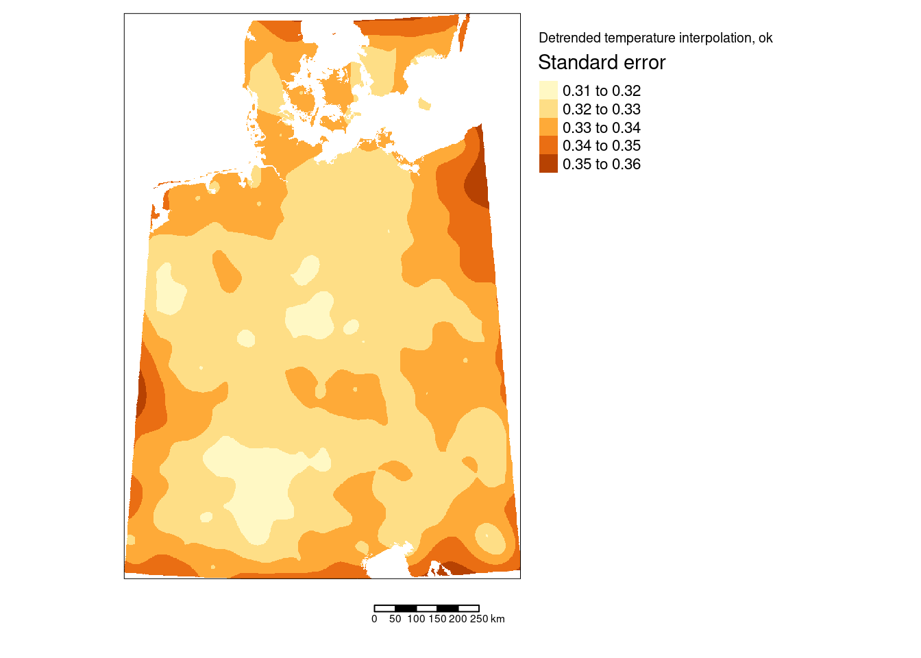
The two areas with slightly higher temperatures are located around Dresden and in the Ruhrgebiet. The areas with lower temperatures seem to be associated with mountainous regions in Switzerland and Austria but also with a region around Metz and around the frankonian swiz.
tm_shape(predTempNoTrendRas %>% subset(subset="var1.var")) +
tm_raster(col="var1.var", title = "Standard error") +
tm_scale_bar() +
tm_layout(title = "Detrended temperature interpolation, ok",
legend.outside = TRUE, attr.outside = TRUE)## ## ── tmap v3 code detected ───────────────────────────────────────────────────────## [v3->v4] `tm_raster()`: migrate the argument(s) related to the legend of the
## visual variable `col` namely 'title' to 'col.legend = tm_legend(<HERE>)'
## ! `tm_scale_bar()` is deprecated. Please use `tm_scalebar()` instead.
## [v3->v4] `tm_layout()`: use `tm_title()` instead of `tm_layout(title = )`
## [plot mode] fit legend/component: Some legend items or map compoments do not
## fit well, and are therefore rescaled.
## ℹ Set the tmap option `component.autoscale = FALSE` to disable rescaling.
The standard errors are much smaller than the kriging estimates. Largest prediction uncertainties occurred to the borders of the interpolated areas - which is expected as we have less data and are therefore more uncertain. Inside of our area of interest we nevertheless also observe some areas with higher uncertainties. It might be worth to explore if these are due to temperature stations with more missing data, shorter recording periods or if those were shots down already some time ago.
But we leave this for now and add the effect of elevation and temperature to the prediction.
As the elevation raster is bigger than the interpolated raster (due to no-data cells) we need to crop the elevation raster.
# get coordinates for all raster cells
xras <- predTempNoTrendRas %>% subset(1)
xras[] <- NA
yras <- xras
xras[] <- coordinates(xras)[,1]
yras[] <- coordinates(xras)[,2]
predTempMan <- subset(predTempNoTrendRas, subset= "var1.pred") +
crop(raster(elev), predTempNoTrendRas) * coef(g)[2] +
xras * coef(g)[3] + yras * coef(g)[4]#tmap_mode("plot")
tm_shape(predTempMan) +
tm_raster(col="layer", title = "Prediction [°C]", n=9,
legend.reverse = TRUE, palette = "-RdBu") +
tm_shape(tempStations) +
tm_symbols(col="YEAR", title.col = "Observed [°C]",
legend.col.reverse = TRUE, palette = "-BrBG",
border.col = "black", size=.1, alpha=.9) +
tm_scale_bar() +
tm_layout(title = "Temperature interpolation, manually handeled trend",
legend.outside = TRUE, attr.outside = TRUE)## ## ── tmap v3 code detected ───────────────────────────────────────────────────────## [v3->v4] `tm_tm_raster()`: migrate the argument(s) related to the scale of the
## visual variable `col` namely 'n', 'palette' (rename to 'values') to col.scale =
## tm_scale(<HERE>).
## [v3->v4] `tm_raster()`: migrate the argument(s) related to the legend of the
## visual variable `col` namely 'title', 'legend.reverse' (rename to 'reverse') to
## 'col.legend = tm_legend(<HERE>)'
## [v3->v4] `tm_symbols()`: migrate the argument(s) related to the scale of the
## visual variable `fill` namely 'palette' (rename to 'values') to fill.scale =
## tm_scale(<HERE>).
## [v3->v4] `symbols()`: use `fill_alpha` instead of `alpha`.
## [v3->v4] `symbols()`: migrate the argument(s) related to the legend of the
## visual variable `fill` namely 'title.col' (rename to 'title') to 'fill.legend =
## tm_legend(<HERE>)'
## ! `tm_scale_bar()` is deprecated. Please use `tm_scalebar()` instead.
## [v3->v4] `tm_layout()`: use `tm_title()` instead of `tm_layout(title = )`
## [scale] tm_raster:() the data variable assigned to 'col' contains positive and negative values, so midpoint is set to 0. Set 'midpoint = NA' in 'fill.scale = tm_scale_intervals(<HERE>)' to use all visual values (e.g. colors)
##
## [cols4all] color palettes: use palettes from the R package cols4all. Run
## `cols4all::c4a_gui()` to explore them. The old palette name "-RdBu" is named
## "rd_bu" (in long format "brewer.rd_bu")
## Multiple palettes called "br_bg" found: "brewer.br_bg", "matplotlib.br_bg". The first one, "brewer.br_bg", is returned.
##
## [scale] tm_symbols:() the data variable assigned to 'fill' contains positive and negative values, so midpoint is set to 0. Set 'midpoint = NA' in 'fill.scale = tm_scale_intervals(<HERE>)' to use all visual values (e.g. colors)
##
## [cols4all] color palettes: use palettes from the R package cols4all. Run
## `cols4all::c4a_gui()` to explore them. The old palette name "-BrBG" is named
## "br_bg" (in long format "brewer.br_bg")
## [plot mode] fit legend/component: Some legend items or map compoments do not
## fit well, and are therefore rescaled.
## ℹ Set the tmap option `component.autoscale = FALSE` to disable rescaling.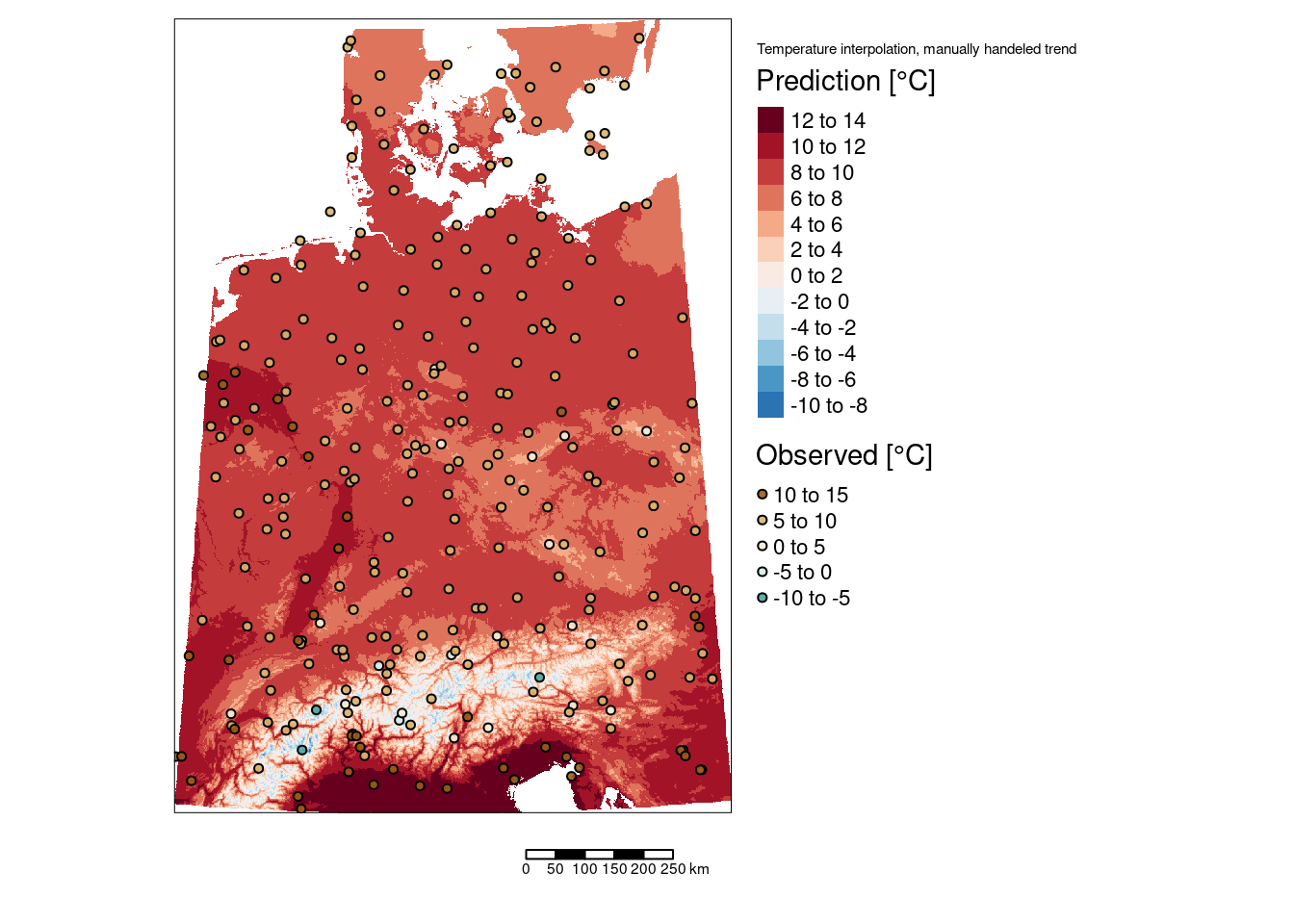
14.4.4 Universal kriging
Universal kriging, also called external drift kriging integrates the trend directly into kriging. Instead of manually detrending and reintegration of the trend after the interpolation, we can directly specify a model that involves the coordinates and covariates.

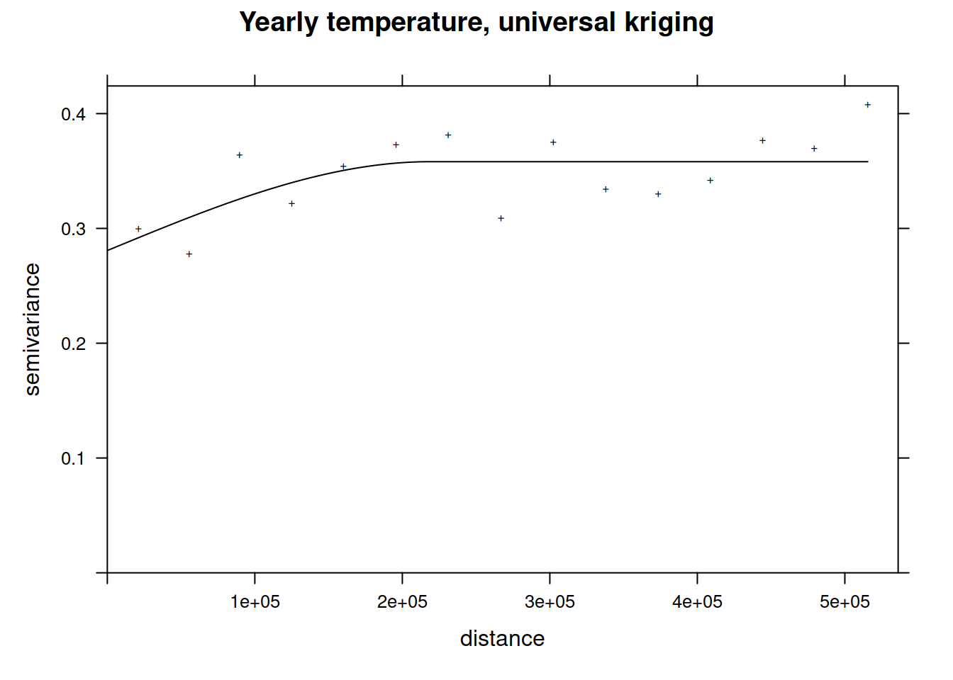
tempUk.vgm <- fit.variogram(tempUk.svar,
model=vgm(model="Sph", nugget = 0.1),
fit.ranges=TRUE)
tempUk.vgm## model psill range
## 1 Nug 0.28072120 0.0
## 2 Sph 0.07741156 218941.3Let’s compare that with the manually detrended empirical variogram:
##   model      psill    range
## 1   Nug 0.28072120      0.0
## 2 Sph 0.07741156 218941.3Same same, no difference. So we could spare use the effort of detrending the data and use univeral kriging directly.
To apply the universal kriging model we need to make sure that all data needed are available and named as expected (as in the variagram model, e.g. ELEV, X and Y) in the predLocations sp object.
names(predLocations) <- "ELEV"
predLocXY <- coordinates(predLocations)
predLocations$X <- predLocXY[,1]
predLocations$Y <- predLocXY[,2]
predTempUk <- krige(YEAR ~ ELEV + X + Y,
locations = as(tempStations, "Spatial"),
newdata = predLocations, model = tempUk.vgm)## [using universal kriging]#tmap_mode("plot")
tm_shape(subset(predTempUkRas, subset = "var1.pred")) +
tm_raster(col="var1.pred", title = "Prediction [°C]", n=9,
legend.reverse = TRUE, palette = "-RdBu") +
tm_shape(tempStations) +
tm_symbols(col="YEAR", title.col = "Observed [°C]",
legend.col.reverse = TRUE, palette = "-BrBG",
border.col = "black", size=.1, alpha=.9) +
tm_scale_bar() +
tm_layout(title = "Temperature interpolation, uk",
legend.outside = TRUE, attr.outside = TRUE)## ## ── tmap v3 code detected ───────────────────────────────────────────────────────## [v3->v4] `tm_tm_raster()`: migrate the argument(s) related to the scale of the
## visual variable `col` namely 'n', 'palette' (rename to 'values') to col.scale =
## tm_scale(<HERE>).
## [v3->v4] `tm_raster()`: migrate the argument(s) related to the legend of the
## visual variable `col` namely 'title', 'legend.reverse' (rename to 'reverse') to
## 'col.legend = tm_legend(<HERE>)'
## [v3->v4] `tm_symbols()`: migrate the argument(s) related to the scale of the
## visual variable `fill` namely 'palette' (rename to 'values') to fill.scale =
## tm_scale(<HERE>).
## [v3->v4] `symbols()`: use `fill_alpha` instead of `alpha`.
## [v3->v4] `symbols()`: migrate the argument(s) related to the legend of the
## visual variable `fill` namely 'title.col' (rename to 'title') to 'fill.legend =
## tm_legend(<HERE>)'
## ! `tm_scale_bar()` is deprecated. Please use `tm_scalebar()` instead.
## [v3->v4] `tm_layout()`: use `tm_title()` instead of `tm_layout(title = )`
## [scale] tm_raster:() the data variable assigned to 'col' contains positive and negative values, so midpoint is set to 0. Set 'midpoint = NA' in 'fill.scale = tm_scale_intervals(<HERE>)' to use all visual values (e.g. colors)
##
## [cols4all] color palettes: use palettes from the R package cols4all. Run
## `cols4all::c4a_gui()` to explore them. The old palette name "-RdBu" is named
## "rd_bu" (in long format "brewer.rd_bu")
## Multiple palettes called "br_bg" found: "brewer.br_bg", "matplotlib.br_bg". The first one, "brewer.br_bg", is returned.
##
## [scale] tm_symbols:() the data variable assigned to 'fill' contains positive and negative values, so midpoint is set to 0. Set 'midpoint = NA' in 'fill.scale = tm_scale_intervals(<HERE>)' to use all visual values (e.g. colors)
##
## [cols4all] color palettes: use palettes from the R package cols4all. Run
## `cols4all::c4a_gui()` to explore them. The old palette name "-BrBG" is named
## "br_bg" (in long format "brewer.br_bg")
For the standard error we need to take the square root of the prediction variance.
#tmap_mode("plot")
tm_shape(subset(predTempUkRas, subset = "var1.var") %>% sqrt()) +
  tm_raster(col="layer", title = "Standard error [°C]", n=9, palette = "Purples") +
  tm_shape(tempStations) +
  tm_symbols(col="YEAR", title.col = "Observed [°C]", palette = "-BrBG",
             border.col = "black", size=.1, alpha=.9) +
  tm_scale_bar() +
  tm_layout(title = "Temperature interpolation, uk",
            legend.outside = TRUE, attr.outside = TRUE)
## ## ── tmap v3 code detected ───────────────────────────────────────────────────────## [v3->v4] `tm_tm_raster()`: migrate the argument(s) related to the scale of the
## visual variable `col` namely 'n', 'palette' (rename to 'values') to col.scale =
## tm_scale(<HERE>).
## [v3->v4] `tm_raster()`: migrate the argument(s) related to the legend of the
## visual variable `col` namely 'title' to 'col.legend = tm_legend(<HERE>)'
## [v3->v4] `tm_symbols()`: migrate the argument(s) related to the scale of the
## visual variable `fill` namely 'palette' (rename to 'values') to fill.scale =
## tm_scale(<HERE>).
## [v3->v4] `symbols()`: use `fill_alpha` instead of `alpha`.
## [v3->v4] `symbols()`: migrate the argument(s) related to the legend of the
## visual variable `fill` namely 'title.col' (rename to 'title') to 'fill.legend =
## tm_legend(<HERE>)'
## ! `tm_scale_bar()` is deprecated. Please use `tm_scalebar()` instead.
## [v3->v4] `tm_layout()`: use `tm_title()` instead of `tm_layout(title = )`
## [cols4all] color palettes: use palettes from the R package cols4all. Run
## `cols4all::c4a_gui()` to explore them. The old palette name "Purples" is named
## "brewer.purples"
## Multiple palettes called "br_bg" found: "brewer.br_bg", "matplotlib.br_bg". The first one, "brewer.br_bg", is returned.
##
## [scale] tm_symbols:() the data variable assigned to 'fill' contains positive and negative values, so midpoint is set to 0. Set 'midpoint = NA' in 'fill.scale = tm_scale_intervals(<HERE>)' to use all visual values (e.g. colors)
##
## [cols4all] color palettes: use palettes from the R package cols4all. Run
## `cols4all::c4a_gui()` to explore them. The old palette name "-BrBG" is named
## "br_bg" (in long format "brewer.br_bg")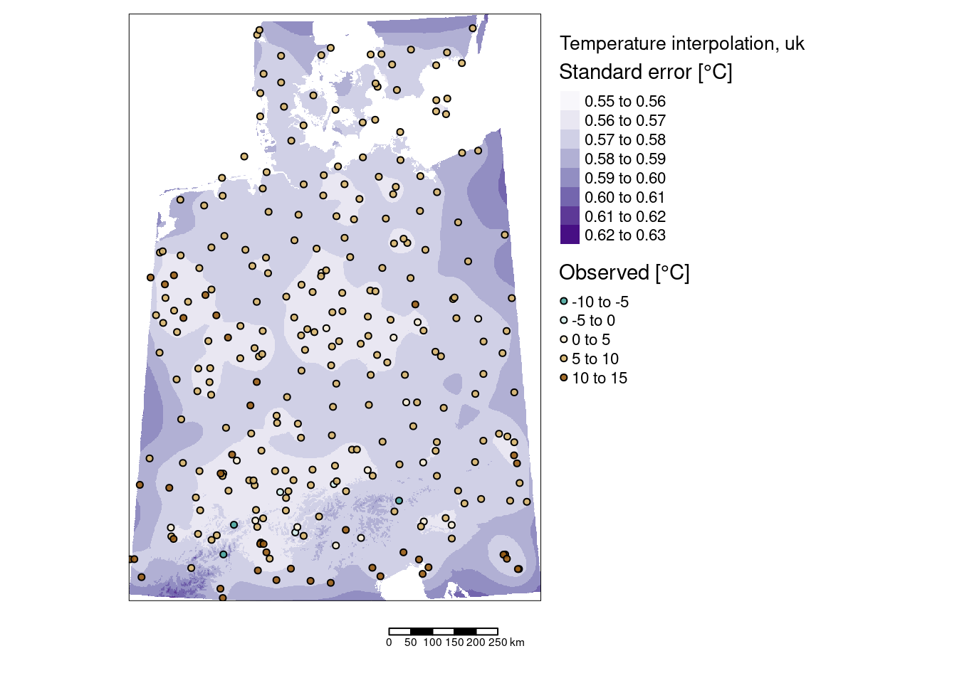
On the first look the prediction looks similar. Let’s check more carefully by differencing the two predictions. For the prediction we use the prediction by the universal kriging approach and the prediction of the ordinary kriging with the reintegrated trend.
There are subtle differences but in the order of hundredths of °C.
tm_shape(diffUkManPred) +
  tm_raster(col="layer", title = "Diff in predicton [°C]",
            n=9, palette = "-RdBu") +
  tm_scale_bar() +
  tm_layout(main.title = "Temperature interpolation,\nuk - manual trend removal",
            legend.outside = TRUE, attr.outside = TRUE)
## ## ── tmap v3 code detected ───────────────────────────────────────────────────────## [v3->v4] `tm_tm_raster()`: migrate the argument(s) related to the scale of the
## visual variable `col` namely 'n', 'palette' (rename to 'values') to col.scale =
## tm_scale(<HERE>).
## [v3->v4] `tm_raster()`: migrate the argument(s) related to the legend of the
## visual variable `col` namely 'title' to 'col.legend = tm_legend(<HERE>)'
## ! `tm_scale_bar()` is deprecated. Please use `tm_scalebar()` instead.
## [v3->v4] `tm_layout()`: use `tm_title()` instead of `tm_layout(main.title = )`
## [scale] tm_raster:() the data variable assigned to 'col' contains positive and negative values, so midpoint is set to 0. Set 'midpoint = NA' in 'fill.scale = tm_scale_intervals(<HERE>)' to use all visual values (e.g. colors)
##
## [cols4all] color palettes: use palettes from the R package cols4all. Run
## `cols4all::c4a_gui()` to explore them. The old palette name "-RdBu" is named
## "rd_bu" (in long format "brewer.rd_bu")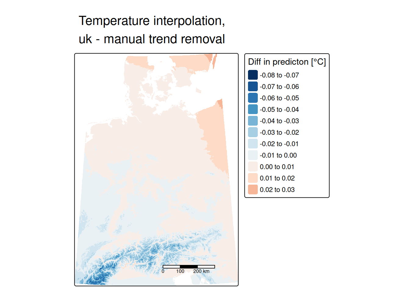
For the standard error comparison we can directly take the result of the ordinary krining as we assumed n addition uncertainty due to the reintegration of the trend.
diffUkManStdErr <- subset(predTempUkRas, subset = "var1.var") - subset(predTempNoTrendRas, subset = "var1.var")For the standard errors we see some minor differences, mostly in the Alps and at the edge of the interpolation area.
tm_shape(diffUkManStdErr) +
  tm_raster(col="layer", title = "Diff in standard error [°C]",
            n=9, palette = "-RdBu") +
  tm_scale_bar() +
  tm_layout(main.title = "Temperature interpolation,\nuk - manual trend removal",
            legend.outside = TRUE, attr.outside = TRUE)
## ## ── tmap v3 code detected ───────────────────────────────────────────────────────## [v3->v4] `tm_tm_raster()`: migrate the argument(s) related to the scale of the
## visual variable `col` namely 'n', 'palette' (rename to 'values') to col.scale =
## tm_scale(<HERE>).
## [v3->v4] `tm_raster()`: migrate the argument(s) related to the legend of the
## visual variable `col` namely 'title' to 'col.legend = tm_legend(<HERE>)'
## ! `tm_scale_bar()` is deprecated. Please use `tm_scalebar()` instead.
## [v3->v4] `tm_layout()`: use `tm_title()` instead of `tm_layout(main.title = )`
## [cols4all] color palettes: use palettes from the R package cols4all. Run
## `cols4all::c4a_gui()` to explore them. The old palette name "-RdBu" is named
## "rd_bu" (in long format "brewer.rd_bu")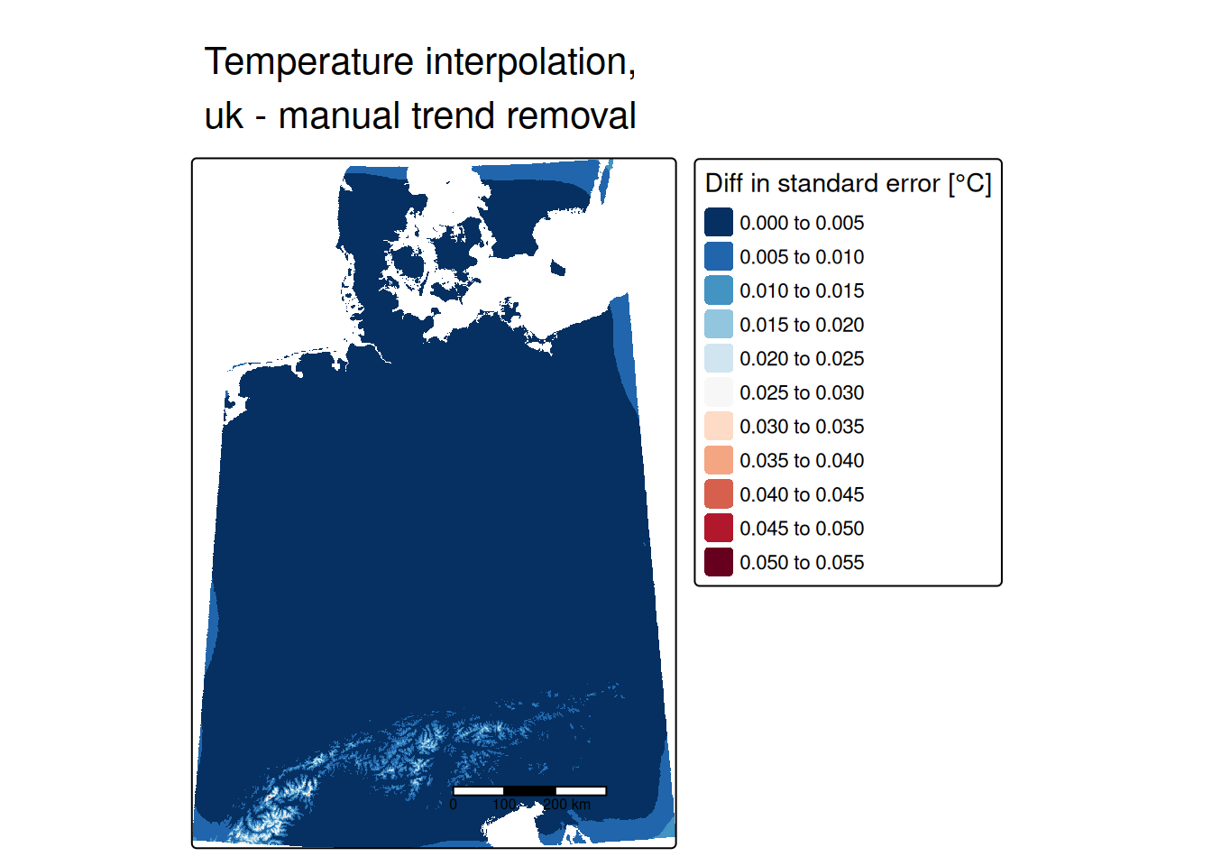
14.4.5 Geostatistical simulation
A problem with kriging is that it tends to over-smooths reality. This effects especially processes that exhibits a nugget effect in the
variogram model. The kriging predictor is the “best linear unbiased predictor” (BLUP) at each point, but the resulting field is commonly smoother than in reality. This might cause problems when using the prediction in further analysis steps and it also provides a distorted view of nature to decision-makers. A more realistic visualization of reality is achieved by the use of conditional geostatistical simulations: the sample points are taken as known, but the interpolated points reproduce the variogram model including the local noise introduced by the nugget effect. The krige method in gstat can also be used to generate simulations, if the optional nsim (“number of simulations”) argument is used. It is interesting to create several ‘alternate realities’, each of which is equally-probable.
As the simulation is computationally expensive we are aggregating the raster for the prediction to 5 by 5km. In addition, we could use the parameters nmax, maxdist and nmin to ease to computational cost.
elev5km <- aggregate(elev, fact=10, fun=mean)

predLocations5km <- as.points(elev5km) %>% as("Spatial")# rasterToPoints(elev5km, spatial = TRUE )
names(predLocations5km) <- "ELEV"
predLocations5km$X <- coordinates(predLocations5km)[,1]
predLocations5km$Y <- coordinates(predLocations5km)[,2]
gridded(predLocations5km) <- TRUEset.seed(42) # for reproducibility I freeze the random generator by setting a seed
predTempUkSim <- krige(YEAR ~ ELEV + X + Y,
locations = as(tempStations, "Spatial"),
newdata = predLocations5km,
model = tempUk.vgm, nsim = 4, nmax = 100)## drawing 4 GLS realisations of beta...
## [using conditional Gaussian simulation]predTempUkSimBrick <- brick(predTempUkSim)
predTempUk5km <- krige(YEAR ~ ELEV + X + Y,
locations = as(tempStations, "Spatial"),
newdata = predLocations5km, model = tempUk.vgm)## [using universal kriging]tm_shape(predTempUkSimBrick) +
tm_raster(col=paste0("sim", 1:4), title = "Temperature [°C]", n=9, palette = "-RdBu",
legend.reverse = TRUE, midpoint = 0) +
tm_scale_bar() +
tm_layout(main.title = "Simulated temparatures",
legend.outside = TRUE, attr.outside = TRUE)## ## ── tmap v3 code detected ───────────────────────────────────────────────────────## [v3->v4] `tm_tm_raster()`: migrate the argument(s) related to the scale of the
## visual variable `col` namely 'n', 'midpoint', 'palette' (rename to 'values') to
## col.scale = tm_scale(<HERE>).
## ℹ For small multiples, specify a 'tm_scale_' for each multiple, and put them in
## a list: 'col.scale = list(<scale1>, <scale2>, ...)'
## [v3->v4] `tm_raster()`: migrate the argument(s) related to the legend of the
## visual variable `col` namely 'title', 'legend.reverse' (rename to 'reverse') to
## 'col.legend = tm_legend(<HERE>)'
## ! `tm_scale_bar()` is deprecated. Please use `tm_scalebar()` instead.
## [v3->v4] `tm_layout()`: use `tm_title()` instead of `tm_layout(main.title = )`
## [cols4all] color palettes: use palettes from the R package cols4all. Run
## `cols4all::c4a_gui()` to explore them. The old palette name "-RdBu" is named
## "rd_bu" (in long format "brewer.rd_bu")
## [plot mode] fit legend/component: Some legend items or map compoments do not
## fit well, and are therefore rescaled.
## ℹ Set the tmap option `component.autoscale = FALSE` to disable rescaling.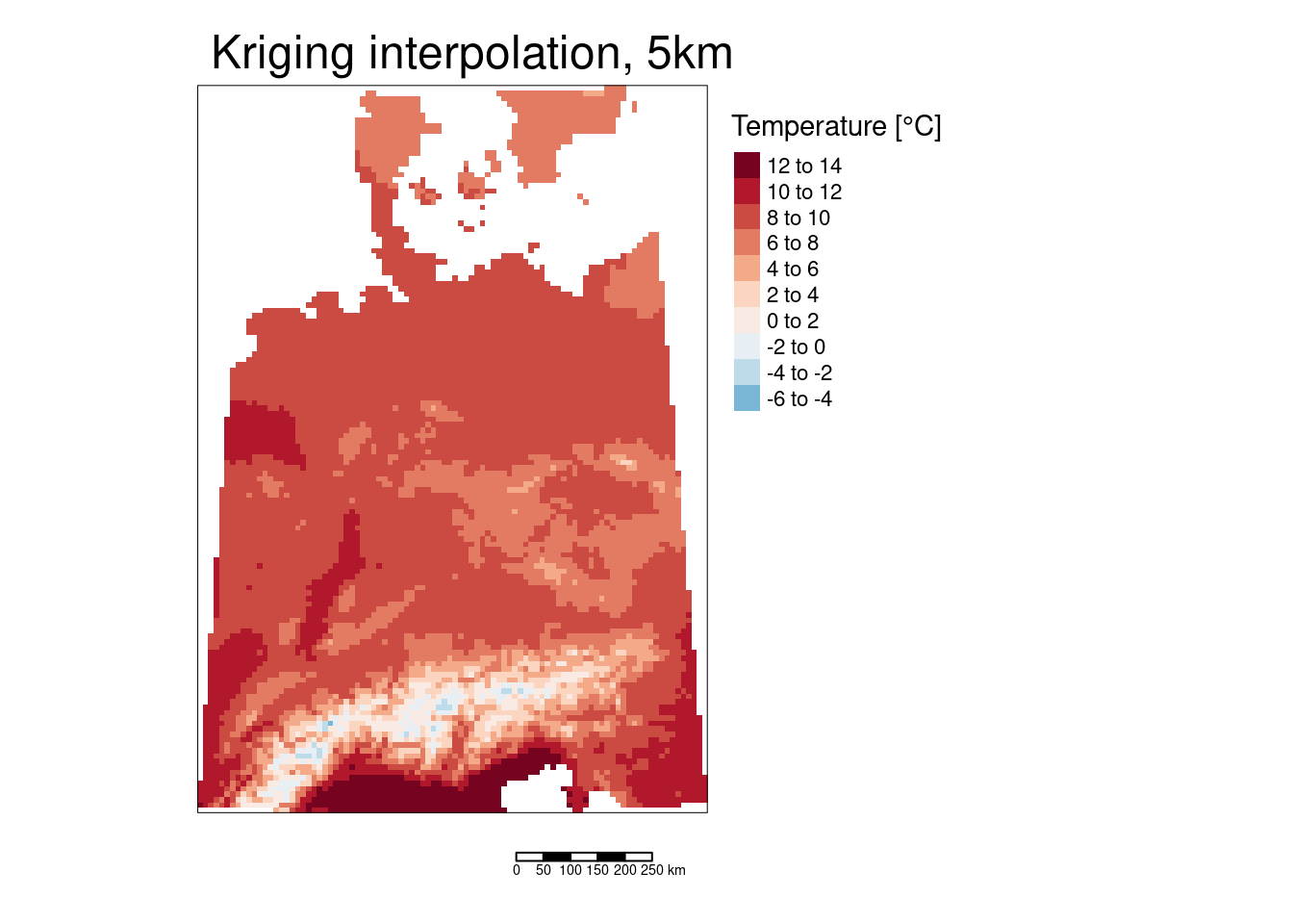
If we compare the simulations with the kriging results we see that they are less smooth and more edgy. While this might not be to important for long term average temperature which can be assumed to be relatively smooth it matters for other processes, such as topsoil heavy metal concentrations.
tm_shape(subset(predTempUk5kmBrick, subset="var1.pred")) +
  tm_raster(col="var1.pred", title = "Temperature [°C]", n=9, palette = "-RdBu",
            legend.reverse = TRUE, midpoint = 0) +
  tm_scale_bar() +
  tm_layout(main.title = "Kriging interpolation, 5km",
            legend.outside = TRUE, attr.outside = TRUE)
## ## ── tmap v3 code detected ───────────────────────────────────────────────────────## [v3->v4] `tm_tm_raster()`: migrate the argument(s) related to the scale of the
## visual variable `col` namely 'n', 'midpoint', 'palette' (rename to 'values') to
## col.scale = tm_scale(<HERE>).
## ℹ For small multiples, specify a 'tm_scale_' for each multiple, and put them in
## a list: 'col.scale = list(<scale1>, <scale2>, ...)'
## [v3->v4] `tm_raster()`: migrate the argument(s) related to the legend of the
## visual variable `col` namely 'title', 'legend.reverse' (rename to 'reverse') to
## 'col.legend = tm_legend(<HERE>)'
## ! `tm_scale_bar()` is deprecated. Please use `tm_scalebar()` instead.
## [v3->v4] `tm_layout()`: use `tm_title()` instead of `tm_layout(main.title = )`
## [cols4all] color palettes: use palettes from the R package cols4all. Run
## `cols4all::c4a_gui()` to explore them. The old palette name "-RdBu" is named
## "rd_bu" (in long format "brewer.rd_bu")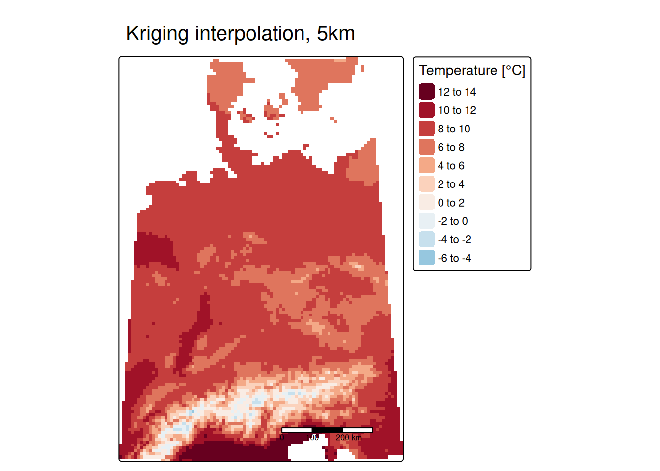
14.4.6 Cross-validation
During the kriging process we had to make quite a couple of decisions which lead to different kriging weights and therefore to different interpolation surfaces. Cross-validation (holding some obervations back, interpolation without them and assessing goodness at the withhold observation locaions) is a commonly used approach to assess goodness of fit for differently models. For performance reason we use the 5km raster.
Say we want to compare the sperical model fitted before with an exponential model - all with a nugget effect. We are using a 5-fold cross-validation approach.
Spherical variogram model
tempSphCv <- krige.cv(YEAR ~ ELEV + X + Y,
                      locations = as(tempStations, "Spatial"),
                      model =  tempUk.vgm, nfold=5)
Exponential variogram model
tempUkExp.vgm <- fit.variogram(tempUk.svar,
                               model=vgm(model="Exp",
                                         nugget = 0.1),
                                 fit.ranges=TRUE)

tempExpCv <- krige.cv(YEAR ~ ELEV + X + Y,
                      locations = as(tempStations, "Spatial"),
                      model =  tempUkExp.vgm, nfold=5)
We can compare the models based on several statistics, based on the residuals (field residual of the cross-validation object).
Mean error (bias), ideally this should be zero.
## [1] -0.001187544## [1] -0.003452224The absolute bias for the spherical model is around 30% smaller than for the exponential model.
Mean square prediction error, ideally 0.
## [1] 0.3220432## [1] 0.3174169The difference her is much smaller and in favor for the exponential model.
correlation observed and predicted, ideally 1
## [1] 0.9799922## [1] 0.9802833correlation predicted and residual, ideally 0
## [1] 0.02370663## [1] 0.02383587If we repeat the cross-validation, we get different results (as long as we do not freeze the random generator). Therefor, it might be useful to repeat the cross-validation several times.
calcCvGof <- function(cvObj, response)
{
  res <- data.frame(bias=NA, mae=NA, rmse=NA,
                    corObsPred = NA, corPredResid=NA,
                    explVar=NA)
  res$bias <- mean(cvObj$residual)
  res$mae <- mean(abs(cvObj$residual))
  res$rmse <- sqrt(mean(cvObj$residual^2))
  res$corObsPred <- cor(cvObj$observed, cvObj$observed - cvObj$residual)
  res$corPredResid <- cor(cvObj$residual, cvObj$observed - cvObj$residual)
  res$explVar <- 1-var(cvObj$residual, na.rm=TRUE)/var(response)
  return(res)
}
cvGof <- NULL
nfold <- 5
response <- tempStations$YEAR
for(i in 1:20)
{
tempSphCv <- krige.cv(YEAR ~ ELEV + X + Y,
locations = as(tempStations, "Spatial"),
model = tempUk.vgm, nfold= nfold, verbose = FALSE)
tempExpCv <- krige.cv(YEAR ~ ELEV + X + Y,
locations = as(tempStations, "Spatial"),
model = tempUkExp.vgm, nfold= nfold, verbose = FALSE)
cvGof1 <- calcCvGof(tempSphCv, response = response)
cvGof1$model <- "Spherical + nugget"
cvGof1$run <- i
cvGof2 <- calcCvGof(tempExpCv, response = response)
cvGof2$model <- "Exponential + nugget"
cvGof2$run <- i
cvGof <- rbind(cvGof, cvGof1, cvGof2)
}p1 <- ggplot(cvGof, aes(x=model, y= rmse)) +
geom_boxplot(notch = TRUE) +
xlab("Variogram model") + ylab("RMSE")
p2 <- ggplot(cvGof, aes(x=model, y= mae)) +
geom_boxplot(notch = TRUE) +
xlab("Variogram model") + ylab("MAE")
p3 <- ggplot(cvGof, aes(x=model, y= bias)) +
geom_boxplot(notch = TRUE) +
xlab("Variogram model") + ylab("Bias")
p4 <- ggplot(cvGof, aes(x=model, y= corPredResid)) + geom_boxplot(notch = TRUE) +
xlab("Variogram model") +
ylab("Cor. pred. vs. resid.")
p5 <- ggplot(cvGof, aes(x=model, y= corObsPred)) + geom_boxplot(notch = TRUE) +
xlab("Variogram model") +
ylab("Cor. obs. vs. pred.")
p6 <- ggplot(cvGof, aes(x=model, y= explVar)) + geom_boxplot(notch = TRUE) +
xlab("Variogram model") +
ylab("Explained variance")
ggpubr::ggarrange(p1,p2,p3, p4, p5, p6)## Notch went outside hinges
## ℹ Do you want `notch = FALSE`?
## Notch went outside hinges
## ℹ Do you want `notch = FALSE`?
## Notch went outside hinges
## ℹ Do you want `notch = FALSE`?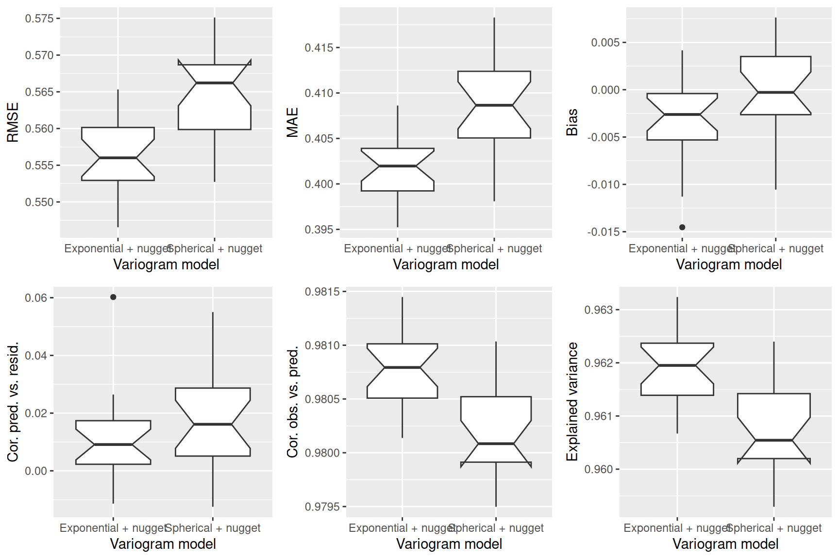
The goodness of fit indicators are slightly in favor of the exponential model. However, the differences are really small.
We get a much clearer picture if we compare a model with and without a nugget effect. However, the differences are still not that big.
cvGof <- NULL
nfold <- 5
response <- tempStations$YEAR
tempUkExpNoNug.vgm <- fit.variogram(tempUk.svar, model=vgm(model="Exp"),
fit.ranges=TRUE)
for(i in 1:20)
{
tempSphCv <- krige.cv(YEAR ~ ELEV + X + Y,
locations = as(tempStations, "Spatial"),
model = tempUk.vgm, nfold= nfold, verbose = FALSE)
tempExpCv <- krige.cv(YEAR ~ ELEV + X + Y,
locations = as(tempStations, "Spatial"),
model = tempUkExpNoNug.vgm, nfold= nfold, verbose = FALSE)
cvGof1 <- calcCvGof(tempSphCv, response = response)
cvGof1$model <- "Exponential + nugget"
cvGof1$run <- i
cvGof2 <- calcCvGof(tempExpCv, response = response)
cvGof2$model <- "Exponential"
cvGof2$run <- i
cvGof <- rbind(cvGof, cvGof1, cvGof2)
}p1 <- ggplot(cvGof, aes(x=model, y= rmse)) +
geom_boxplot(notch = TRUE) +
xlab("Variogram model") + ylab("RMSE")
p2 <- ggplot(cvGof, aes(x=model, y= mae)) +
geom_boxplot(notch = TRUE) +
xlab("Variogram model") + ylab("MAE")
p3 <- ggplot(cvGof, aes(x=model, y= bias)) +
geom_boxplot(notch = TRUE) +
xlab("Variogram model") + ylab("Bias")
p4 <- ggplot(cvGof, aes(x=model, y= corPredResid)) + geom_boxplot(notch = TRUE) +
xlab("Variogram model") +
ylab("Cor. pred. vs. resid.")
p5 <- ggplot(cvGof, aes(x=model, y= corObsPred)) + geom_boxplot(notch = TRUE) +
xlab("Variogram model") +
ylab("Cor. obs. vs. pred.")
p6 <- ggplot(cvGof, aes(x=model, y= explVar)) + geom_boxplot(notch = TRUE) +
xlab("Variogram model") +
ylab("Explained variance")
ggpubr::ggarrange(p1,p2,p3, p4, p5, p6)## Notch went outside hinges
## ℹ Do you want `notch = FALSE`?
## Notch went outside hinges
## ℹ Do you want `notch = FALSE`?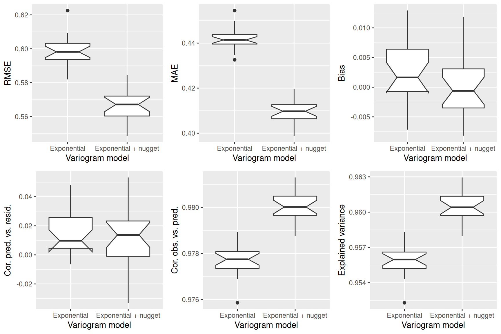
Would the interpolation be much worse if we would use different weights for fitting the variogram? This can be changed by setting fit.method in variogram.fit.
cvGof <- NULL
nfold <- 5
response <- tempStations$YEAR
tempUkExpM6.vgm <- fit.variogram(tempUk.svar, model=vgm(model="Exp"),
fit.ranges=TRUE, fit.method = 6)
tempUkExpM2.vgm <- fit.variogram(tempUk.svar, model=vgm(model="Exp"),
fit.ranges=TRUE, fit.method = 2)
for(i in 1:20)
{
tempExpCv <- krige.cv(YEAR ~ ELEV + X + Y, locations = as(tempStations, "Spatial"),
model = tempUk.vgm, nfold= nfold, verbose = FALSE)
tempExpM2Cv <- krige.cv(YEAR ~ ELEV + X + Y, locations = as(tempStations, "Spatial"),
model = tempUkExpM2.vgm, nfold= nfold, verbose = FALSE)
tempExpM6Cv <- krige.cv(YEAR ~ ELEV + X + Y, locations = as(tempStations, "Spatial"),
model = tempUkExpM6.vgm, nfold= nfold, verbose = FALSE)
cvGof1 <- calcCvGof(tempExpCv, response = response)
cvGof1$model <- "Exponential + nugget, weights= N_j/(h_j^2)"
cvGof1$run <- i
cvGof2 <- calcCvGof(tempExpM2Cv, response = response)
cvGof2$model <- "Exponential+ nugget, weights = N_j"
cvGof2$run <- i
cvGof3 <- calcCvGof(tempExpM6Cv, response = response)
cvGof3$model <- "Exponential+ nugget, weights = 1"
cvGof3$run <- i
cvGof <- rbind(cvGof, cvGof1, cvGof2, cvGof3)
}p1 <- ggplot(cvGof, aes(x=model, y= rmse)) + geom_boxplot(notch = TRUE) +
xlab("Variogram model") + ylab("RMSE") + coord_flip()
p2 <- ggplot(cvGof, aes(x=model, y= mae)) + geom_boxplot(notch = TRUE) +
xlab("Variogram model") + ylab("MAE") + coord_flip() + theme(axis.text.y=element_blank())
p3 <- ggplot(cvGof, aes(x=model, y= bias)) + geom_boxplot(notch = TRUE) +
xlab("Variogram model") + ylab("Bias") + coord_flip() + theme(axis.text.y=element_blank())
p4 <- ggplot(cvGof, aes(x=model, y= corPredResid)) + geom_boxplot(notch = TRUE) +
xlab("Variogram model") + ylab("Cor. pred. vs. resid.") + coord_flip()
p5 <- ggplot(cvGof, aes(x=model, y= corObsPred)) + geom_boxplot(notch = TRUE) +
xlab("Variogram model") + ylab("Cor. obs. vs. pred.") + coord_flip() + theme(axis.text.y=element_blank())
p6 <- ggplot(cvGof, aes(x=model, y= explVar)) + geom_boxplot(notch = TRUE) +
xlab("Variogram model") + ylab("Explained variance") + coord_flip() + theme(axis.text.y= element_blank())
ggpubr::ggarrange(p1,p2,p3, p4, p5, p6, widths = c(1.6,1,1))## Notch went outside hinges
## ℹ Do you want `notch = FALSE`?
## Notch went outside hinges
## ℹ Do you want `notch = FALSE`?
## Notch went outside hinges
## ℹ Do you want `notch = FALSE`?
## Notch went outside hinges
## ℹ Do you want `notch = FALSE`?
## Notch went outside hinges
## ℹ Do you want `notch = FALSE`?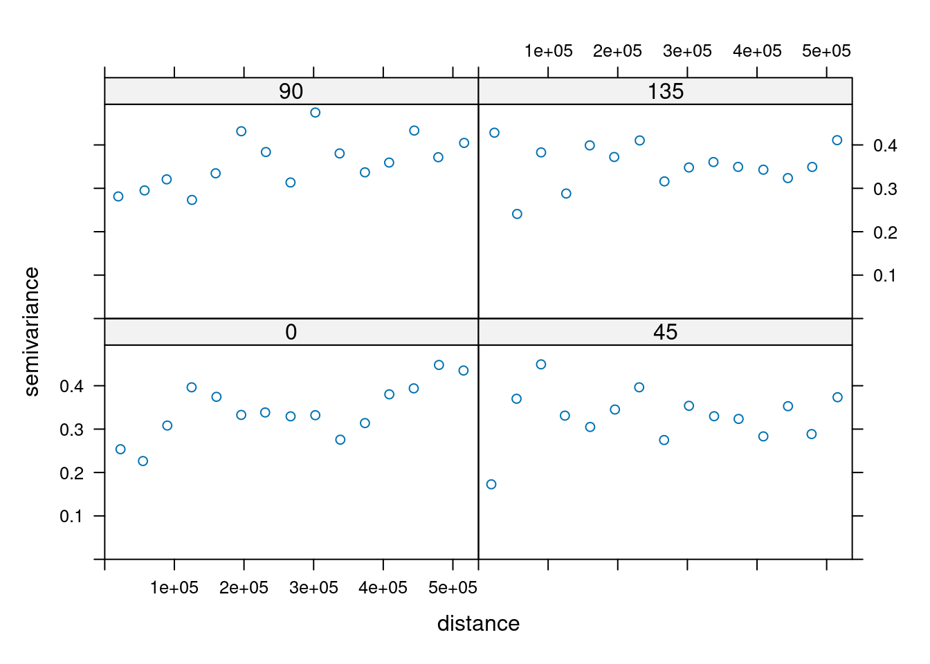
14.4.7 Anisotropy
14.4.7.1 Geometric anisotropy
We start with creating directional empirical variograms. These are specified by the alpha parameter, that we specify here as a vector of length 4 which covers the directions NW-NE, NE-SE, SE-SW, SW-NW. We only need to define half of the range from 0 to 360, as this definition affects as well the corresponding other part of the circle.
tempUk.svarAnis <- variogram(YEAR ~ ELEV + X + Y,
                         alpha= (0:3)*45,
                         data=tempStations)
plot(tempUk.svarAnis)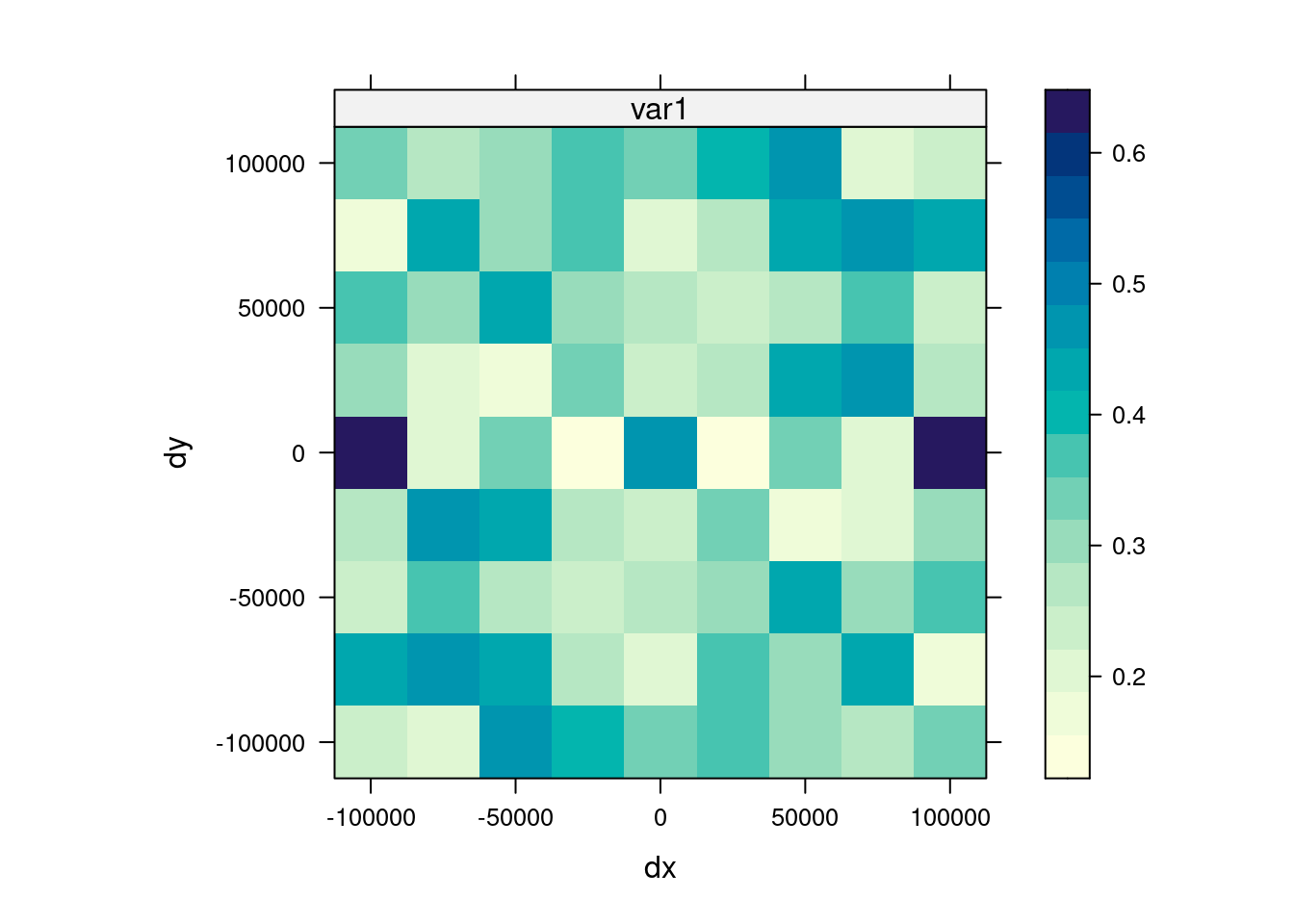
We don’t see much of a difference here. Anisotropy does not seem to be a problem here.
Let’s next plot a variogram map
tempUk.svarMap <- variogram(YEAR ~ ELEV + X + Y,
                         map= TRUE,
                         cutoff = 10^5, width = 25*10^3,
                         data=tempStations)
plot(tempUk.svarMap)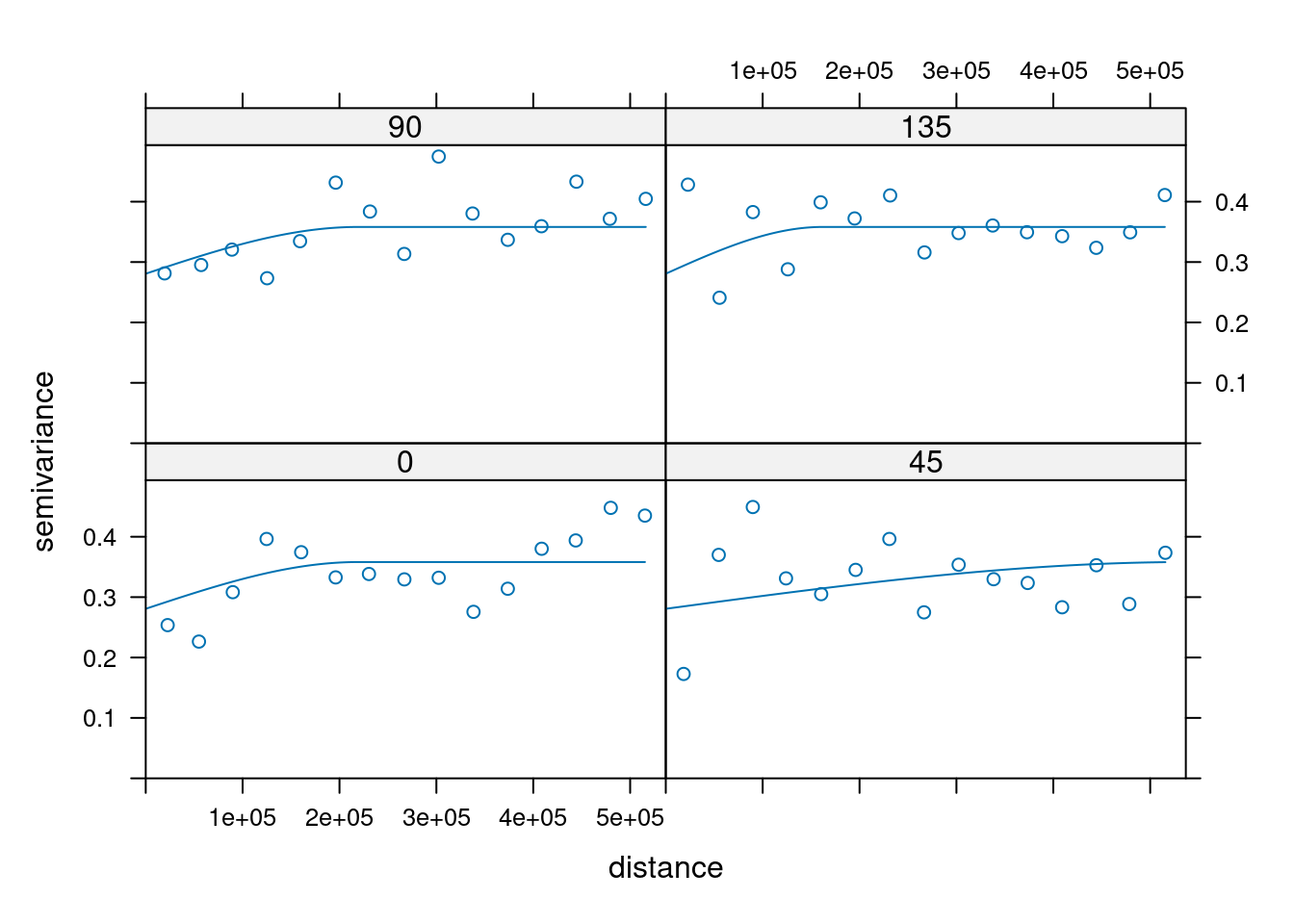
tempUk.vgmAnis <- fit.variogram(
                    tempUk.svar, model=
                      vgm(model="Sph", nugget = NA,
                          anis = c(45,0.3)),
                    fit.ranges=TRUE)
plot(tempUk.svarAnis, tempUk.vgmAnis)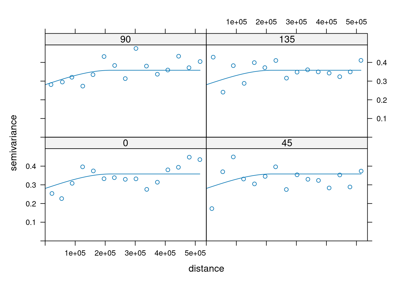
As a contrast the variogram fitted without anisotropy:
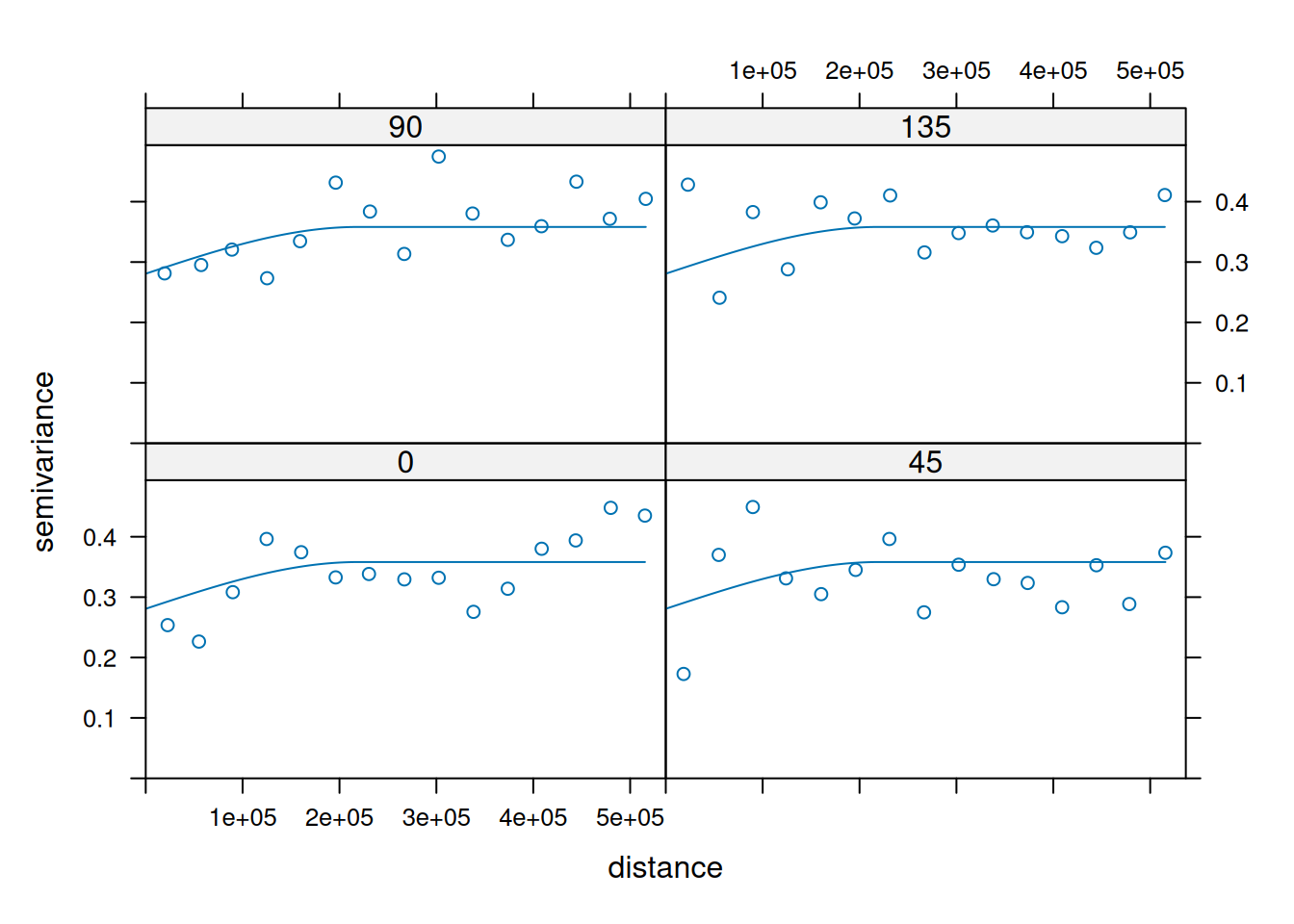
14.4.8 Block kriging
14.4.8.1 Regular blocks
We use the 5 km raster for the prediction and a 50 x 50 km regular block size.
predTempUkBlock <- krige(YEAR ~ ELEV + X + Y,
                    locations = as(tempStations, "Spatial"),
                    newdata = predLocations5km, model =  tempUk.vgm,
                    block = c(5*10^5, 5*10^5))
## [using universal kriging]Let’s compare that to point kriging (as well done at the 5km raster cell size).
predTempUk5km <- krige(YEAR ~ ELEV + X + Y,
                    locations = as(tempStations, "Spatial"),
                    newdata = predLocations5km, model =  tempUk.vgm)
## [using universal kriging]mapUk5kmBlock <- tm_shape(subset(predTempUkBlockRas, subset = "var1.pred")) +
tm_raster(col="var1.pred", title = "Prediction [°C]", n=9,
legend.reverse = TRUE, palette = "-RdBu") +
tm_shape(tempStations) +
tm_symbols(col="YEAR", title.col = "Observed [°C]",
legend.col.reverse = TRUE, palette = "-BrBG",
border.col = "black", size=.1, alpha=.9) +
tm_scale_bar() +
tm_layout(title = "Temperature interpolation, block uk",
legend.outside = TRUE, attr.outside = TRUE)## ## ── tmap v3 code detected ───────────────────────────────────────────────────────## [v3->v4] `tm_tm_raster()`: migrate the argument(s) related to the scale of the
## visual variable `col` namely 'n', 'palette' (rename to 'values') to col.scale =
## tm_scale(<HERE>).
## [v3->v4] `tm_raster()`: migrate the argument(s) related to the legend of the
## visual variable `col` namely 'title', 'legend.reverse' (rename to 'reverse') to
## 'col.legend = tm_legend(<HERE>)'
## [v3->v4] `tm_symbols()`: migrate the argument(s) related to the scale of the
## visual variable `fill` namely 'palette' (rename to 'values') to fill.scale =
## tm_scale(<HERE>).
## [v3->v4] `symbols()`: use `fill_alpha` instead of `alpha`.
## [v3->v4] `symbols()`: migrate the argument(s) related to the legend of the
## visual variable `fill` namely 'title.col' (rename to 'title') to 'fill.legend =
## tm_legend(<HERE>)'
## ! `tm_scale_bar()` is deprecated. Please use `tm_scalebar()` instead.
## [v3->v4] `tm_layout()`: use `tm_title()` instead of `tm_layout(title = )`For the standard error we need to take the square root of the prediction variance.
#tmap_mode("plot")
mapUkStderr5kmBlock <- tm_shape(subset(predTempUkBlockRas, subset = "var1.var") %>% sqrt()) +
  tm_raster(col="layer", title = "Standard error [°C]", n=9, palette = "Purples") +
  tm_shape(tempStations) +
  tm_symbols(col="YEAR", title.col = "Observed [°C]", palette = "-BrBG",
             border.col = "black", size=.1, alpha=.9) +
  tm_scale_bar() +
  tm_layout(title = "Temperature interpolation, block uk",
            legend.outside = TRUE, attr.outside = TRUE)
## [v3->v4] `tm_raster()`: migrate the argument(s) related to the legend of the
## visual variable `col` namely 'title' to 'col.legend = tm_legend(<HERE>)'
## [v3->v4] `symbols()`: use `fill_alpha` instead of `alpha`.
## [v3->v4] `symbols()`: migrate the argument(s) related to the legend of the
## visual variable `fill` namely 'title.col' (rename to 'title') to 'fill.legend =
## tm_legend(<HERE>)'
## ! `tm_scale_bar()` is deprecated. Please use `tm_scalebar()` instead.
## [v3->v4] `tm_layout()`: use `tm_title()` instead of `tm_layout(title = )`mapUkStderr5km <- tm_shape(subset(predTempUk5kmRas, subset = "var1.var") %>% sqrt()) +
tm_raster(col="layer", title = "Standard error [°C]", n=9, palette = "Purples") +
tm_shape(tempStations) +
tm_symbols(col="YEAR", title.col = "Observed [°C]", palette = "-BrBG",
border.col = "black", size=.1, alpha=.9) +
tm_scale_bar() +
tm_layout(title = "Temperature interpolation, uk",
legend.outside = TRUE, attr.outside = TRUE)## [v3->v4] `tm_raster()`: migrate the argument(s) related to the legend of the
## visual variable `col` namely 'title' to 'col.legend = tm_legend(<HERE>)'
## [v3->v4] `symbols()`: use `fill_alpha` instead of `alpha`.
## [v3->v4] `symbols()`: migrate the argument(s) related to the legend of the
## visual variable `fill` namely 'title.col' (rename to 'title') to 'fill.legend =
## tm_legend(<HERE>)'
## ! `tm_scale_bar()` is deprecated. Please use `tm_scalebar()` instead.
## [v3->v4] `tm_layout()`: use `tm_title()` instead of `tm_layout(title = )`## [cols4all] color palettes: use palettes from the R package cols4all. Run
## `cols4all::c4a_gui()` to explore them. The old palette name "Purples" is named
## "brewer.purples"
## Multiple palettes called "br_bg" found: "brewer.br_bg", "matplotlib.br_bg". The first one, "brewer.br_bg", is returned.
##
## [scale] tm_symbols:() the data variable assigned to 'fill' contains positive and negative values, so midpoint is set to 0. Set 'midpoint = NA' in 'fill.scale = tm_scale_intervals(<HERE>)' to use all visual values (e.g. colors)
##
## [cols4all] color palettes: use palettes from the R package cols4all. Run
## `cols4all::c4a_gui()` to explore them. The old palette name "-BrBG" is named
## "br_bg" (in long format "brewer.br_bg")
## [plot mode] fit legend/component: Some legend items or map compoments do not
## fit well, and are therefore rescaled.
## ℹ Set the tmap option `component.autoscale = FALSE` to disable rescaling.
## [cols4all] color palettes: use palettes from the R package cols4all. Run
## `cols4all::c4a_gui()` to explore them. The old palette name "Purples" is named
## "brewer.purples"
## Multiple palettes called "br_bg" found: "brewer.br_bg", "matplotlib.br_bg". The first one, "brewer.br_bg", is returned.
##
## [scale] tm_symbols:() the data variable assigned to 'fill' contains positive and negative values, so midpoint is set to 0. Set 'midpoint = NA' in 'fill.scale = tm_scale_intervals(<HERE>)' to use all visual values (e.g. colors)
##
## [cols4all] color palettes: use palettes from the R package cols4all. Run
## `cols4all::c4a_gui()` to explore them. The old palette name "-BrBG" is named
## "br_bg" (in long format "brewer.br_bg")
## [plot mode] fit legend/component: Some legend items or map compoments do not
## fit well, and are therefore rescaled.
## ℹ Set the tmap option `component.autoscale = FALSE` to disable rescaling.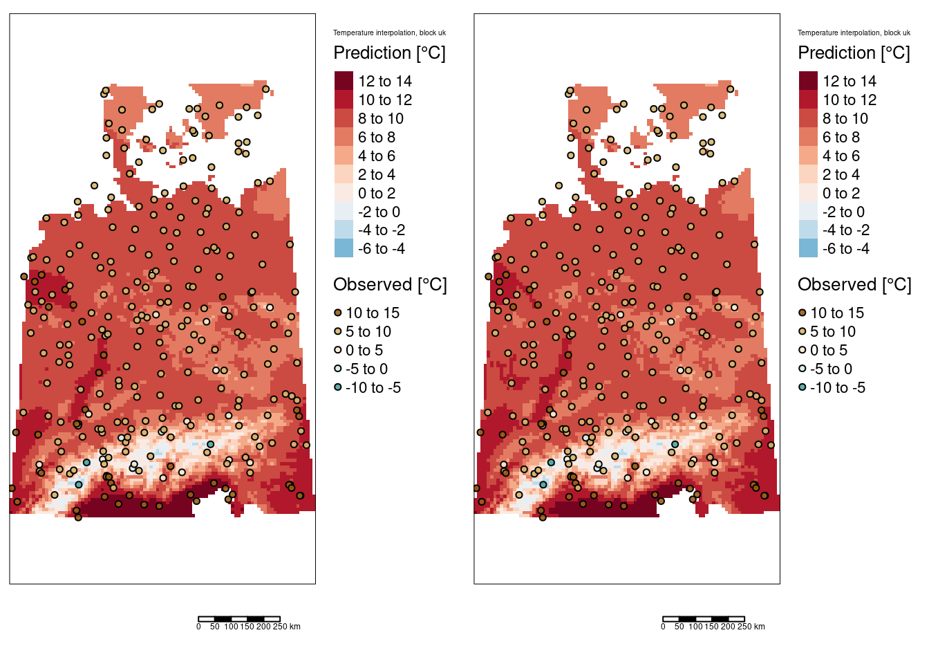
As expected, the standard error for the block kriging are much lower than for the point kriging, as the errors cancel out for the blocks.
mapUk5km <- tm_shape(subset(predTempUk5kmRas, subset = "var1.pred")) +
  tm_raster(col="var1.pred", title = "Prediction [°C]", n=9,
            legend.reverse = TRUE, palette = "-RdBu") +
  tm_shape(tempStations) +
  tm_symbols(col="YEAR", title.col = "Observed [°C]",
             legend.col.reverse = TRUE, palette = "-BrBG",
             border.col = "black", size=.1, alpha=.9) +
  tm_scale_bar() +
  tm_layout(title = "Temperature interpolation, block uk",
            legend.outside = TRUE, attr.outside = TRUE)
## ## ── tmap v3 code detected ───────────────────────────────────────────────────────## [v3->v4] `tm_tm_raster()`: migrate the argument(s) related to the scale of the
## visual variable `col` namely 'n', 'palette' (rename to 'values') to col.scale =
## tm_scale(<HERE>).
## [v3->v4] `tm_raster()`: migrate the argument(s) related to the legend of the
## visual variable `col` namely 'title', 'legend.reverse' (rename to 'reverse') to
## 'col.legend = tm_legend(<HERE>)'
## [v3->v4] `tm_symbols()`: migrate the argument(s) related to the scale of the
## visual variable `fill` namely 'palette' (rename to 'values') to fill.scale =
## tm_scale(<HERE>).
## [v3->v4] `symbols()`: use `fill_alpha` instead of `alpha`.
## [v3->v4] `symbols()`: migrate the argument(s) related to the legend of the
## visual variable `fill` namely 'title.col' (rename to 'title') to 'fill.legend =
## tm_legend(<HERE>)'
## ! `tm_scale_bar()` is deprecated. Please use `tm_scalebar()` instead.
## [v3->v4] `tm_layout()`: use `tm_title()` instead of `tm_layout(title = )`## [scale] tm_raster:() the data variable assigned to 'col' contains positive and negative values, so midpoint is set to 0. Set 'midpoint = NA' in 'fill.scale = tm_scale_intervals(<HERE>)' to use all visual values (e.g. colors)
## [cols4all] color palettes: use palettes from the R package cols4all. Run
## `cols4all::c4a_gui()` to explore them. The old palette name "-RdBu" is named
## "rd_bu" (in long format "brewer.rd_bu")Multiple palettes called "br_bg" found: "brewer.br_bg", "matplotlib.br_bg". The first one, "brewer.br_bg", is returned.
## [scale] tm_symbols:() the data variable assigned to 'fill' contains positive and negative values, so midpoint is set to 0. Set 'midpoint = NA' in 'fill.scale = tm_scale_intervals(<HERE>)' to use all visual values (e.g. colors)
## [cols4all] color palettes: use palettes from the R package cols4all. Run
## `cols4all::c4a_gui()` to explore them. The old palette name "-BrBG" is named
## "br_bg" (in long format "brewer.br_bg")[plot mode] fit legend/component: Some legend items or map compoments do not
## fit well, and are therefore rescaled.
## ℹ Set the tmap option `component.autoscale = FALSE` to disable rescaling.[scale] tm_raster:() the data variable assigned to 'col' contains positive and negative values, so midpoint is set to 0. Set 'midpoint = NA' in 'fill.scale = tm_scale_intervals(<HERE>)' to use all visual values (e.g. colors)
## [cols4all] color palettes: use palettes from the R package cols4all. Run
## `cols4all::c4a_gui()` to explore them. The old palette name "-RdBu" is named
## "rd_bu" (in long format "brewer.rd_bu")Multiple palettes called "br_bg" found: "brewer.br_bg", "matplotlib.br_bg". The first one, "brewer.br_bg", is returned.
## [scale] tm_symbols:() the data variable assigned to 'fill' contains positive and negative values, so midpoint is set to 0. Set 'midpoint = NA' in 'fill.scale = tm_scale_intervals(<HERE>)' to use all visual values (e.g. colors)
## [cols4all] color palettes: use palettes from the R package cols4all. Run
## `cols4all::c4a_gui()` to explore them. The old palette name "-BrBG" is named
## "br_bg" (in long format "brewer.br_bg")[plot mode] fit legend/component: Some legend items or map compoments do not
## fit well, and are therefore rescaled.
## ℹ Set the tmap option `component.autoscale = FALSE` to disable rescaling.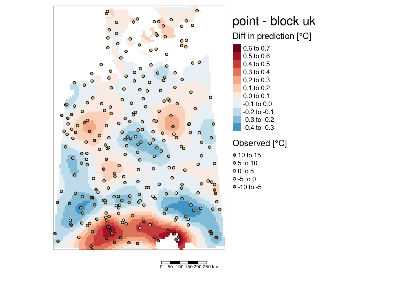
The predicted temperature maps do not show much of a difference.
predDiff <- predTempUk5kmRas$var1.pred - predTempUkBlockRas$var1.pred

tm_shape(predDiff) +
  tm_raster(col="layer", title = "Diff in prediction [°C]", n=9,
            legend.reverse = TRUE, palette = "-RdBu") +
  tm_shape(tempStations) +
  tm_symbols(col="YEAR", title.col = "Observed [°C]",
             legend.col.reverse = TRUE, palette = "-BrBG",
             border.col = "black", size=.1, alpha=.9) +
  tm_scale_bar() +
  tm_layout(title = "point - block uk",
            legend.outside = TRUE, attr.outside = TRUE)
## ## ── tmap v3 code detected ───────────────────────────────────────────────────────## [v3->v4] `tm_tm_raster()`: migrate the argument(s) related to the scale of the
## visual variable `col` namely 'n', 'palette' (rename to 'values') to col.scale =
## tm_scale(<HERE>).
## [v3->v4] `tm_raster()`: migrate the argument(s) related to the legend of the
## visual variable `col` namely 'title', 'legend.reverse' (rename to 'reverse') to
## 'col.legend = tm_legend(<HERE>)'
## [v3->v4] `tm_symbols()`: migrate the argument(s) related to the scale of the
## visual variable `fill` namely 'palette' (rename to 'values') to fill.scale =
## tm_scale(<HERE>).
## [v3->v4] `symbols()`: use `fill_alpha` instead of `alpha`.
## [v3->v4] `symbols()`: migrate the argument(s) related to the legend of the
## visual variable `fill` namely 'title.col' (rename to 'title') to 'fill.legend =
## tm_legend(<HERE>)'
## ! `tm_scale_bar()` is deprecated. Please use `tm_scalebar()` instead.
## [v3->v4] `tm_layout()`: use `tm_title()` instead of `tm_layout(title = )`
## [scale] tm_raster:() the data variable assigned to 'col' contains positive and negative values, so midpoint is set to 0. Set 'midpoint = NA' in 'fill.scale = tm_scale_intervals(<HERE>)' to use all visual values (e.g. colors)
##
## [cols4all] color palettes: use palettes from the R package cols4all. Run
## `cols4all::c4a_gui()` to explore them. The old palette name "-RdBu" is named
## "rd_bu" (in long format "brewer.rd_bu")
## Multiple palettes called "br_bg" found: "brewer.br_bg", "matplotlib.br_bg". The first one, "brewer.br_bg", is returned.
##
## [scale] tm_symbols:() the data variable assigned to 'fill' contains positive and negative values, so midpoint is set to 0. Set 'midpoint = NA' in 'fill.scale = tm_scale_intervals(<HERE>)' to use all visual values (e.g. colors)
##
## [cols4all] color palettes: use palettes from the R package cols4all. Run
## `cols4all::c4a_gui()` to explore them. The old palette name "-BrBG" is named
## "br_bg" (in long format "brewer.br_bg")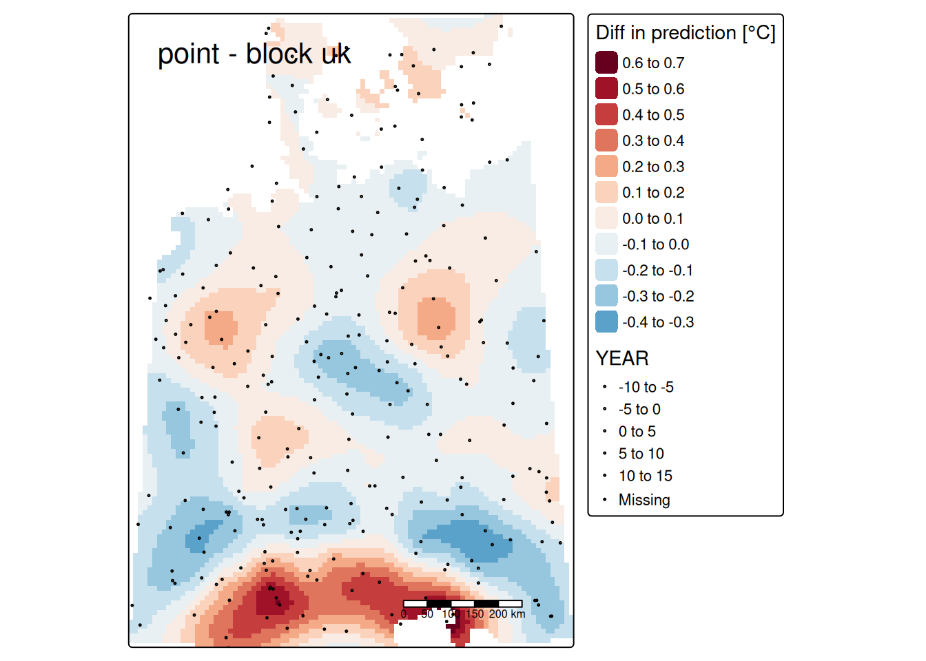
14.5 Case study: heavy metal concentrations in the Meuse floodplain
We use a dataset that comes with the gstat package. See ?meuse for the description of the attributes of the data.frame.
This data set gives locations and topsoil heavy metal concentrations, along with a number of soil and landscape variables at the observation locations, collected in a flood plain of the river Meuse, near the village of Stein (NL). Heavy metal concentrations are from composite samples of an area of approximately 15 m x 15 m.
Make spatial and assign appropriate CRS (Rijksdriehoek (RDH) (Netherlands topographical) map coordinates):
## Warning in CPL_crs_from_input(x): GDAL Message 1: +init=epsg:XXXX syntax is
## deprecated. It might return a CRS with a non-EPSG compliant axis order.## cadmium copper lead zinc
## Min. : 0.200 Min. : 14.00 Min. : 37.0 Min. : 113.0
## 1st Qu.: 0.800 1st Qu.: 23.00 1st Qu.: 72.5 1st Qu.: 198.0
## Median : 2.100 Median : 31.00 Median :123.0 Median : 326.0
## Mean : 3.246 Mean : 40.32 Mean :153.4 Mean : 469.7
## 3rd Qu.: 3.850 3rd Qu.: 49.50 3rd Qu.:207.0 3rd Qu.: 674.5
## Max. :18.100 Max. :128.00 Max. :654.0 Max. :1839.0
##
## elev dist om ffreq soil lime
## Min. : 5.180 Min. :0.00000 Min. : 1.000 1:84 1:97 0:111
## 1st Qu.: 7.546 1st Qu.:0.07569 1st Qu.: 5.300 2:48 2:46 1: 44
## Median : 8.180 Median :0.21184 Median : 6.900 3:23 3:12
## Mean : 8.165 Mean :0.24002 Mean : 7.478
## 3rd Qu.: 8.955 3rd Qu.:0.36407 3rd Qu.: 9.000
## Max. :10.520 Max. :0.88039 Max. :17.000
## NA's :2
## landuse dist.m
## W :50 Min. : 10.0
## Ah :39 1st Qu.: 80.0
## Am :22 Median : 270.0
## Fw :10 Mean : 290.3
## Ab : 8 3rd Qu.: 450.0
## (Other):25 Max. :1000.0
## NA's : 1The dataset provides topsoil heavy metal concentrations, along with a number of soil and landscape variables at the observation locations, collected in a flood plain of the river Meuse, near the village of Stein in the Netherlands. Heavy metal concentrations are from composite samples of an area of approximately 15 m x 15 m.
Heavy metal concentrations are in mg/kg soil (ppm): cadmium, copper, lead, zinc.
Other variables are (see ?meuse):
elevrelative elevation above local river bed in meterdistdistance to the Meuse; obtained from the nearest cell inmeuse.grid, which in turn was derived by a spread (spatial distance) GIS operation, horizontal precision 20 metres; then normalized to \([0,1]\)dist.mdistance to river Meuse in meters, as obtained during the field surveyomorganic matter, kg (100 kg)-1 soil (percent)ffreqflooding frequency class: 1 = once in two years; 2 = once in ten years; 3 = one in 50 yearssoilsoil type according to the 1:50 000 soil map of the Netherlands. 1 = Rd10A (Calcareous weakly-developed meadow soils, light sandy clay); 2 = Rd90C/VII (Non-calcareous weakly-developed meadow soils, heavy sandy clay to light clay); 3 = Bkd26/VII (Red Brick soil, fine-sandy, silty light clay)limelime class: 0 = absent, 1 = present by field test with 5% HCllanduselanduse class: Aa Agriculture/unspecified = , Ab = Agr/sugar beetsm, Ag = Agr/small grains, Ah = Agr/??, Am = Agr/maize, B = woods, Bw = trees in pasture, DEN = ??, Fh = tall fruit trees, Fl = low fruit trees; Fw = fruit trees in pasture, Ga = home gardens, SPO = sport field, STA = stable yard, Tv = ?? , W = pasture
The dataset is a more useful example for the application of anisotropy and cokriging than the temperature dataset used above.
For interpolation with universal kriging another dataset is of importance, meuse.grid which contains the required covariates.
data(meuse.grid)
coordinates(meuse.grid) = ~x+y
proj4string(meuse.grid) <- CRS("+init=epsg:28992")
gridded(meuse.grid) <-  TRUE
summary(meuse.grid@data)
## part.a part.b dist soil ffreq
## Min. :0.0000 Min. :0.0000 Min. :0.0000 1:1665 1: 779
## 1st Qu.:0.0000 1st Qu.:0.0000 1st Qu.:0.1193 2:1084 2:1335
## Median :0.0000 Median :1.0000 Median :0.2715 3: 354 3: 989
## Mean :0.3986 Mean :0.6014 Mean :0.2971
## 3rd Qu.:1.0000 3rd Qu.:1.0000 3rd Qu.:0.4402
## Max. :1.0000 Max. :1.0000 Max. :0.9926Convert to sf object for plotting in tmap;
Get an OSM background map.
tm_shape(osmbgMeuse) + tm_rgb() +
tm_shape(meuse_sf) +
  tm_bubbles(size="zinc") +
  tm_scalebar() +
  tm_layout(attr.outside = TRUE, legend.outside = TRUE)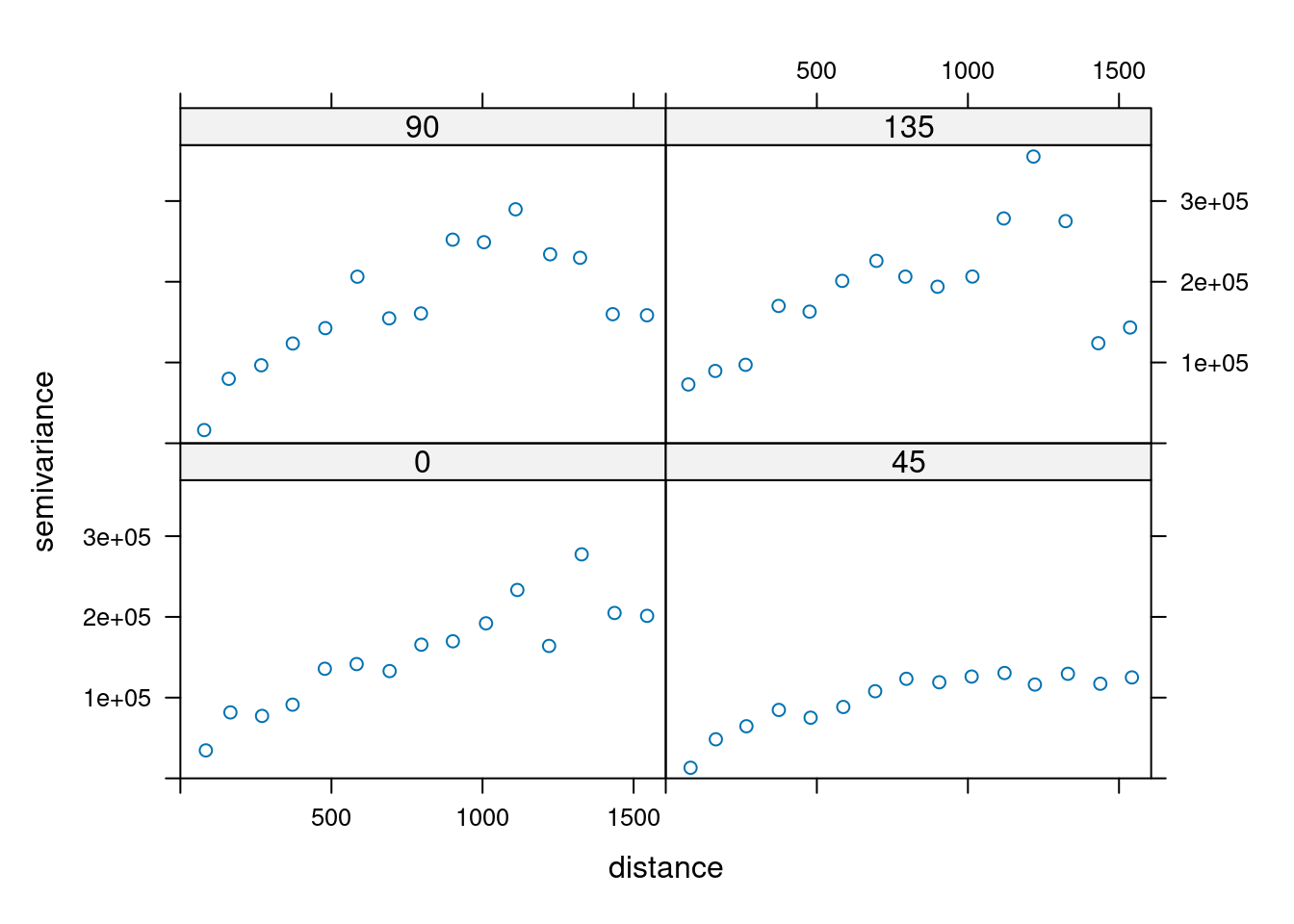
14.5.1 Anisotropy
14.5.1.1 Ordinary kriging
Let’s first look at the variogram map to spot anisotropy for zinc.
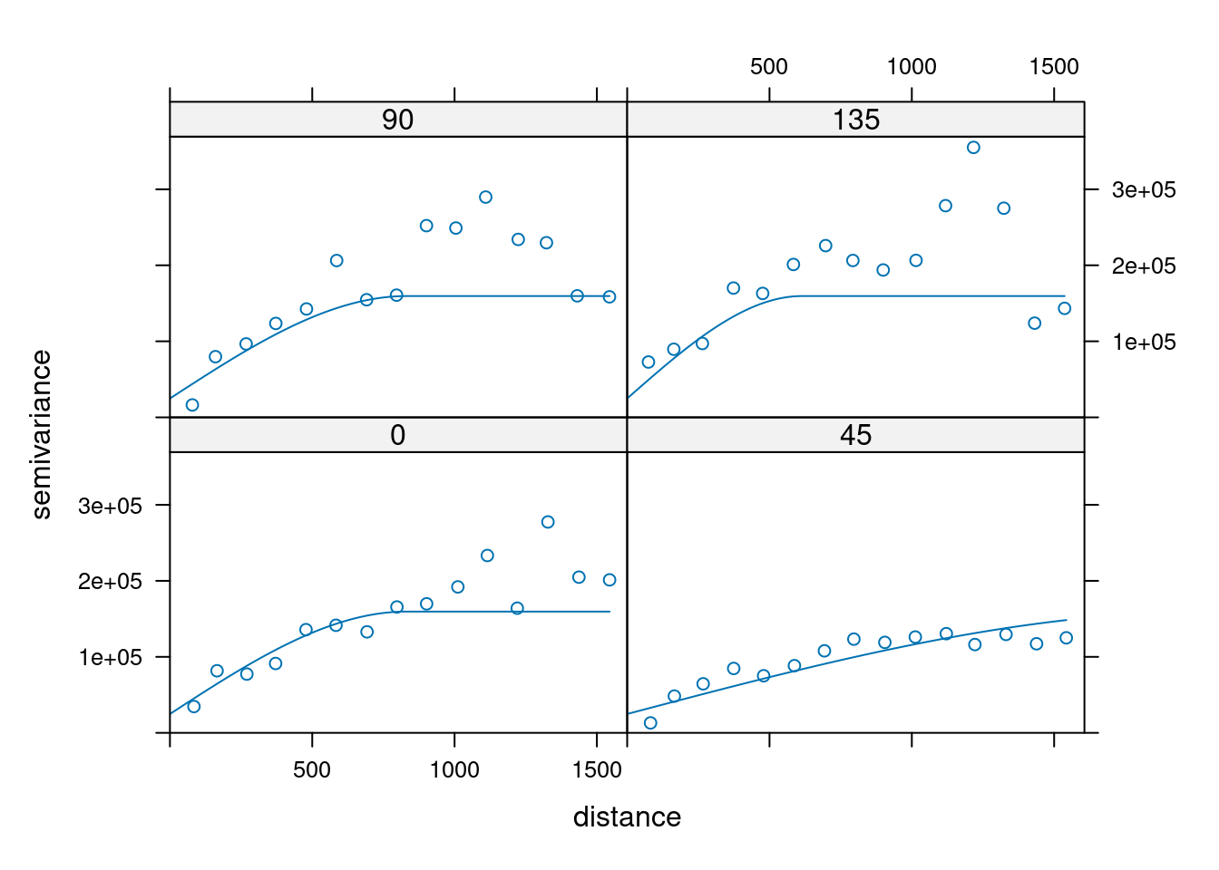
There is clearly an anisotropic effect with the longest range running in SW-NE direction.
Let’s use this information for a directional variogram. We specify the four quadrants (S-N, SW-NE, W-E, NW-SE) by the parameter alpha (in degree).
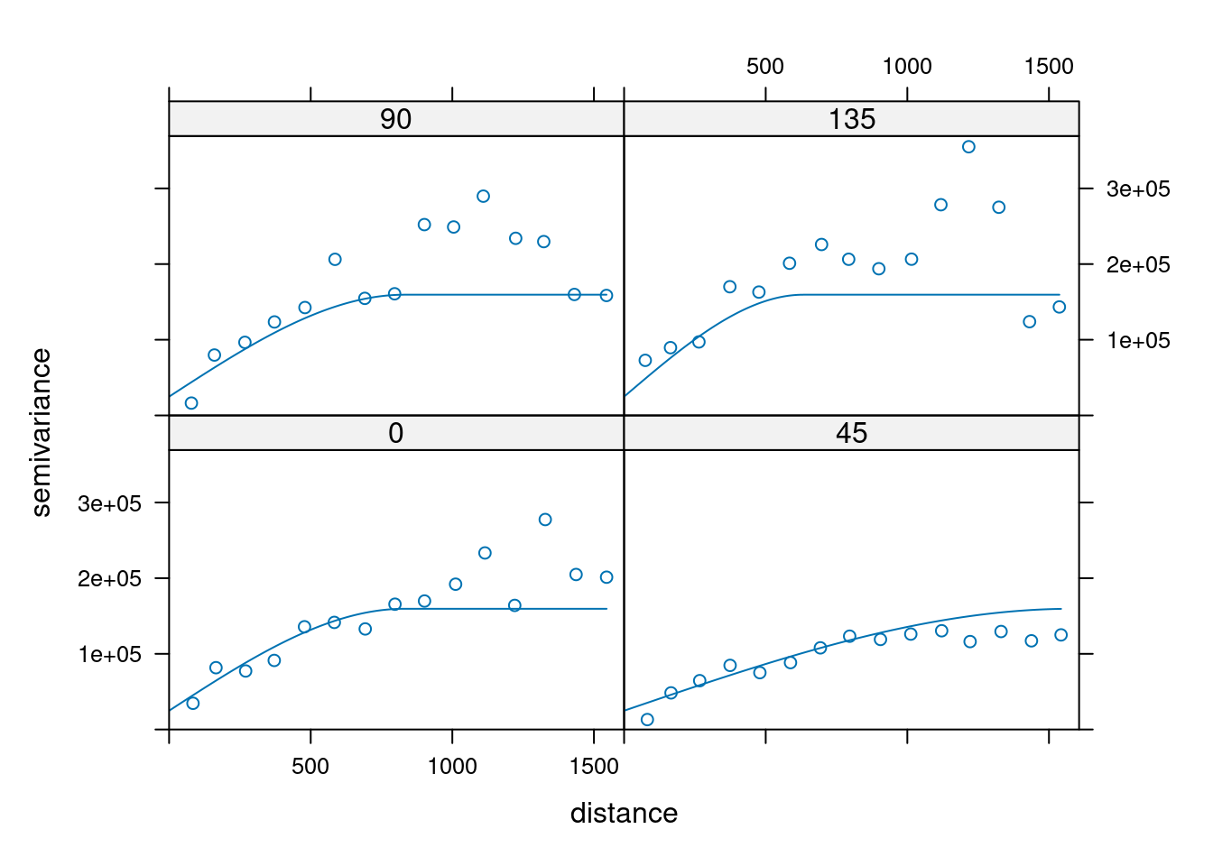
We see that the range in SW-NE direction is much longer than in SE-NW direction. We might estimate that the range in SE-NW direction is shorter by a factor of 0.3 and use this to fit a variogram which considers the anisotropy (parameter anis). The first parameter, 45, refers to the main axis direction: it is the angle for the principal direction of continuity (measured in degrees, clockwise from positive Y, i.e. North). The second parameter, 0.3, is the anisotropy ratio, the ratio of the minor range to the major range (a value between 0 and 1) The sample variogram needs to be an undirectional variogram.
zn.v <- variogram(zinc ~ 1, data= meuse)

zn.vgmAnis <- fit.variogram(
                    zn.v, model=
                      vgm(model="Sph", nugget = NA,
                          anis = c(45,0.3)),
                    fit.ranges=TRUE, fit.sills=TRUE)

plot(zn.v.dir, zn.vgmAnis)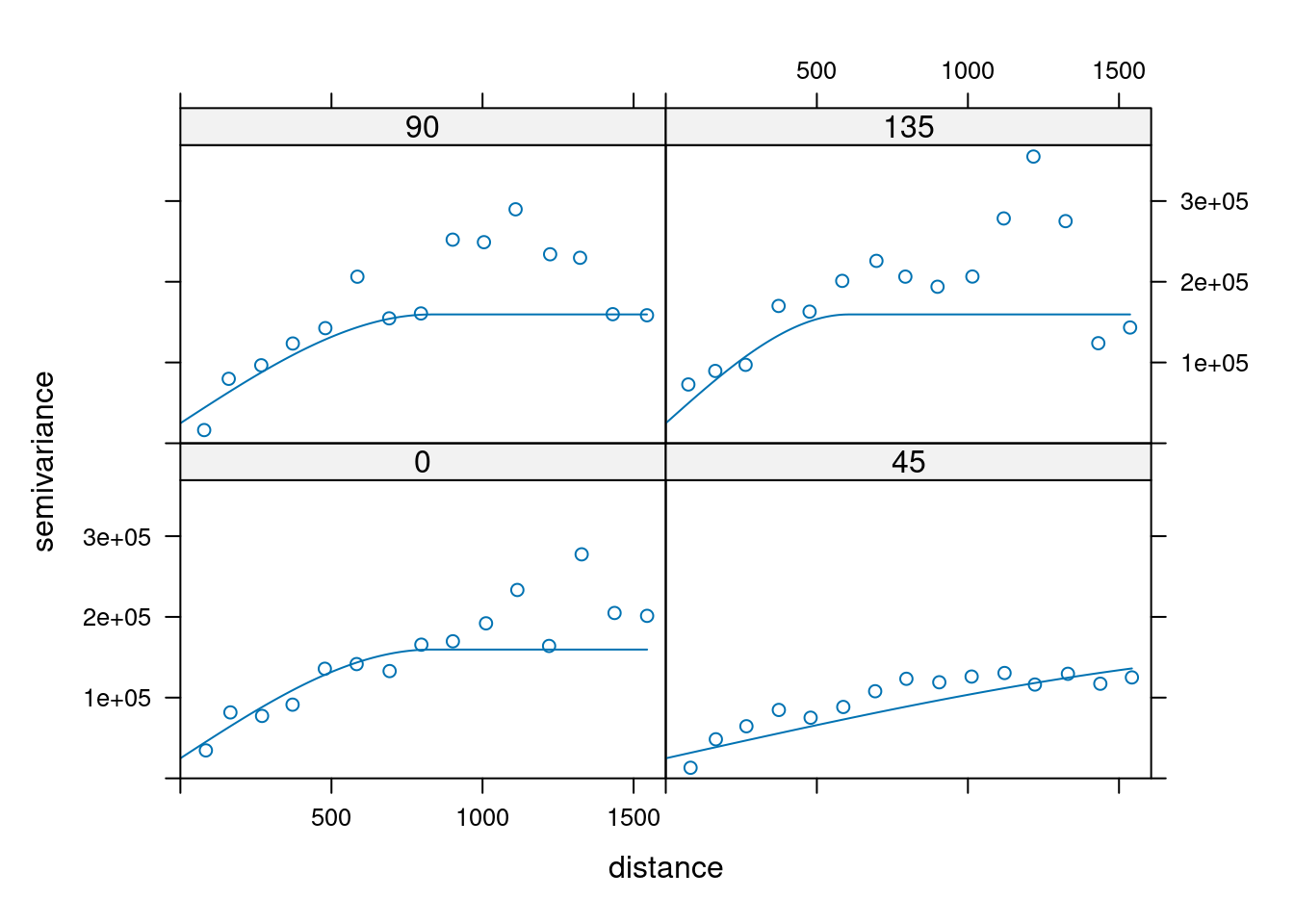
The fitted model has a range in the principal direction (45° , NE) of 2044.8034973, and of 0.3 × 2044.8034973 = 613.4410492 in the minor direction (135°).
Unfortunately, gstat does not allow to estimate the anisotropy parameters. But we can play a bit with the anisotropy parameters. Given the variogram map, the anisotropy ratio seems most promissing.
zn.vgmAnis04 <- fit.variogram(
                    zn.v, model=
                      vgm(model="Sph", nugget = NA,
                          anis = c(45,0.4)),
                    fit.ranges=TRUE, fit.sills=TRUE)

plot(zn.v.dir, zn.vgmAnis04)
zn.vgmAnis025 <- fit.variogram(
                    zn.v, model=
                      vgm(model="Sph", nugget = NA,
                          anis = c(45,0.25)),
                    fit.ranges=TRUE, fit.sills=TRUE)

plot(zn.v.dir, zn.vgmAnis025)
Which of the models should we prefer? Let’s try that by means of 5-fold cross-validation. We use here just one run. Preferable would be the repetition as describe above.
zn.anis03.cv <- krige.cv(zinc ~ 1,
                      locations = meuse,
                      model =  zn.vgmAnis, nfold=5)
zn.anis04.cv <- krige.cv(zinc ~ 1,
                      locations = meuse,
                      model =  zn.vgmAnis04, nfold=5)
zn.anis025.cv <- krige.cv(zinc ~ 1,
                      locations = meuse,
model = zn.vgmAnis025, nfold=5)## [1] 238.116## [1] 248.5612## [1] 236.4387Based on the RMSE the model with the anisotropy range of 0.4 is preferable.
Let’s have a look how the interpolation looks like:
## [using ordinary kriging]tm_shape(subset(predZincOkRas, subset = "var1.pred")) +
tm_raster(col="var1.pred", title = "Prediction [ppm]", n=9,
legend.reverse = TRUE, palette = "Reds") +
tm_shape(meuse_sf) +
tm_bubbles(size="zinc", alpha=0.5) +
tm_scale_bar() +
tm_layout(title = "Zinc, ok",
legend.outside = TRUE, attr.outside = TRUE)## ## ── tmap v3 code detected ───────────────────────────────────────────────────────## [v3->v4] `tm_tm_raster()`: migrate the argument(s) related to the scale of the
## visual variable `col` namely 'n', 'palette' (rename to 'values') to col.scale =
## tm_scale(<HERE>).
## [v3->v4] `tm_raster()`: migrate the argument(s) related to the legend of the
## visual variable `col` namely 'title', 'legend.reverse' (rename to 'reverse') to
## 'col.legend = tm_legend(<HERE>)'
## [v3->v4] `tm_bubbles()`: use `fill_alpha` instead of `alpha`.
## ! `tm_scale_bar()` is deprecated. Please use `tm_scalebar()` instead.
## [v3->v4] `tm_layout()`: use `tm_title()` instead of `tm_layout(title = )`
## [cols4all] color palettes: use palettes from the R package cols4all. Run
## `cols4all::c4a_gui()` to explore them. The old palette name "Reds" is named
## "brewer.reds"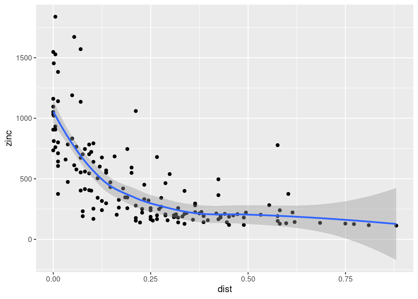
For the standard error we need to take the square root of the prediction variance.
tm_shape(subset(predZincOkRas, subset = "var1.var") %>% sqrt()) +
  tm_raster(col="layer", title = "Standard error [ppm]", n=9, palette = "Purples") +
  tm_shape(meuse_sf) +
  tm_bubbles(size="zinc", alpha=0.5) +
  tm_scale_bar() +
  tm_layout(title = "Zinc, ordinary kriging",
            legend.outside = TRUE, attr.outside = TRUE)
## ## ── tmap v3 code detected ───────────────────────────────────────────────────────## [v3->v4] `tm_tm_raster()`: migrate the argument(s) related to the scale of the
## visual variable `col` namely 'n', 'palette' (rename to 'values') to col.scale =
## tm_scale(<HERE>).
## [v3->v4] `tm_raster()`: migrate the argument(s) related to the legend of the
## visual variable `col` namely 'title' to 'col.legend = tm_legend(<HERE>)'
## [v3->v4] `tm_bubbles()`: use `fill_alpha` instead of `alpha`.
## ! `tm_scale_bar()` is deprecated. Please use `tm_scalebar()` instead.
## [v3->v4] `tm_layout()`: use `tm_title()` instead of `tm_layout(title = )`
## [cols4all] color palettes: use palettes from the R package cols4all. Run
## `cols4all::c4a_gui()` to explore them. The old palette name "Purples" is named
## "brewer.purples"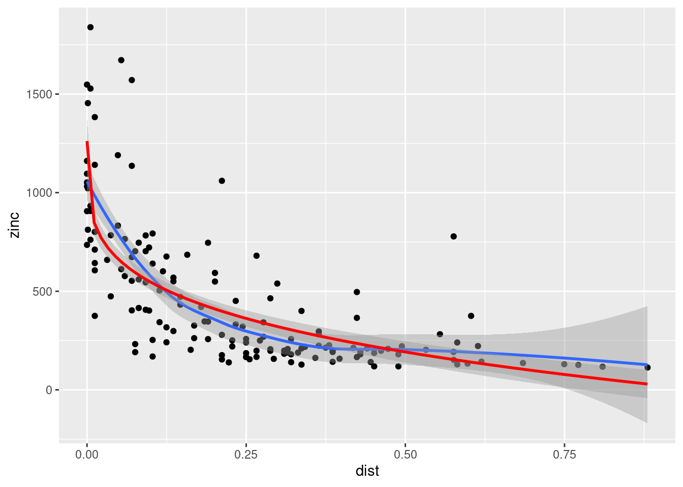
14.5.1.2 Universal kriging
However, universal kriging might be a better option. The map above looked like distance to the river Meuse might be of importance. Let’s check this hypothesis.
## `geom_smooth()` using method = 'loess' and formula = 'y ~ x'
Clearly a non-linear trend. We could try to model that by regressing zinc against some root of distance.
ggplot(meuse@data, mapping = aes(x=dist, y=zinc)) +
geom_point() + geom_smooth() +
geom_smooth(method = lm, formula= y ~ I(x^(1/4)), colour="red")## `geom_smooth()` using method = 'loess' and formula = 'y ~ x'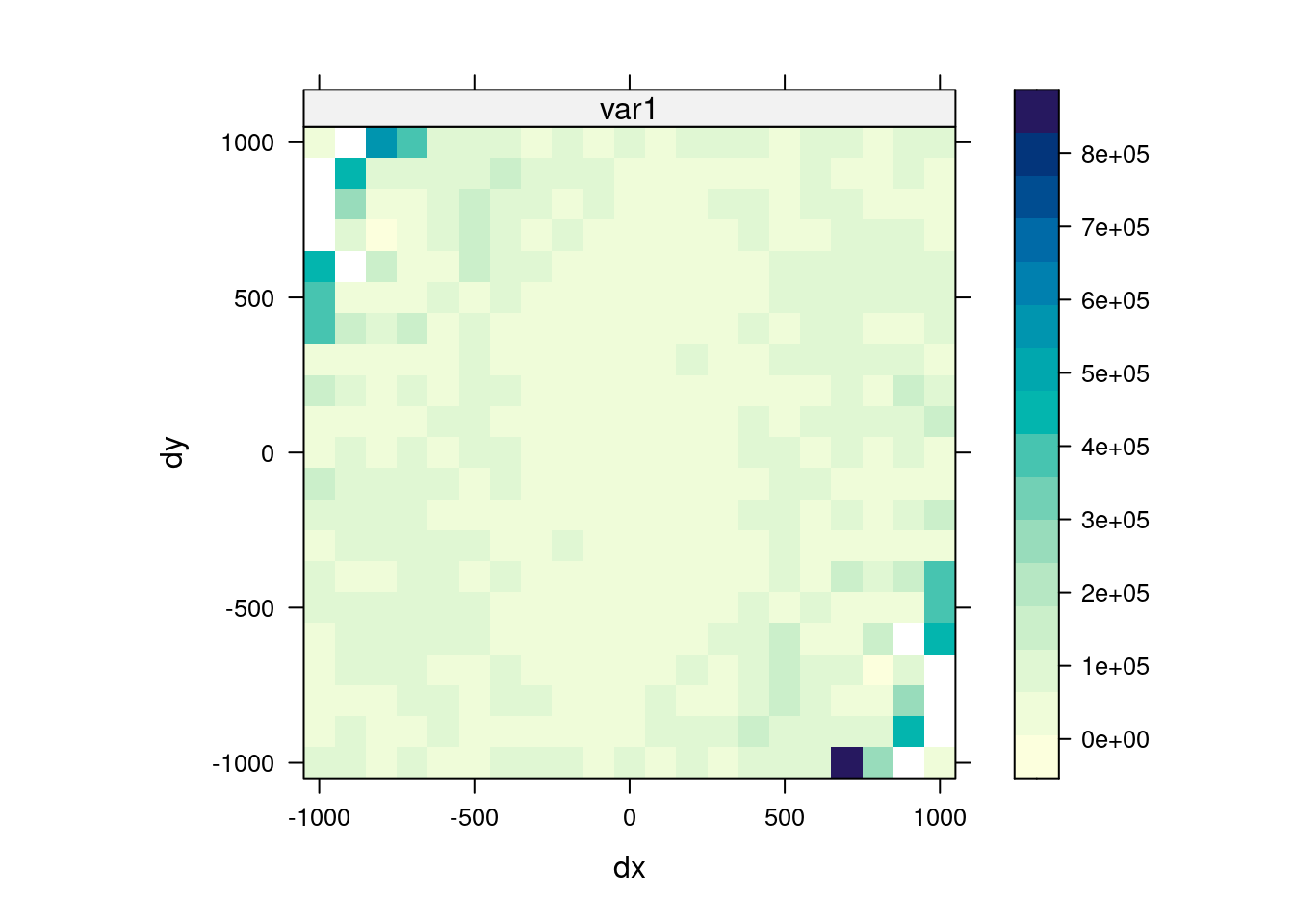
##
## Call:
## lm(formula = zinc ~ I(dist^(1/4)), data = meuse@data)
##
## Residuals:
##     Min      1Q  Median      3Q     Max
## -526.68 -131.59  -42.50   82.61 1022.95
##
## Coefficients:
##               Estimate Std. Error t value Pr(>|t|)
## (Intercept)    1261.68      58.59   21.53   <2e-16 ***
## I(dist^(1/4)) -1272.22      88.85  -14.32   <2e-16 ***
## ---
## Signif. codes:  0 '***' 0.001 '**' 0.01 '*' 0.05 '.' 0.1 ' ' 1
##
## Residual standard error: 240.7 on 153 degrees of freedom
## Multiple R-squared:  0.5726, Adjusted R-squared:  0.5699
## F-statistic:   205 on 1 and 153 DF,  p-value: < 2.2e-16
How does that effect the variogram map?
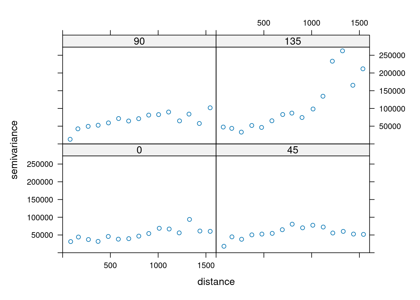
It clearly changed the direction of the longest rnage, which seems now more N-S oriented. Check the directional variogram.
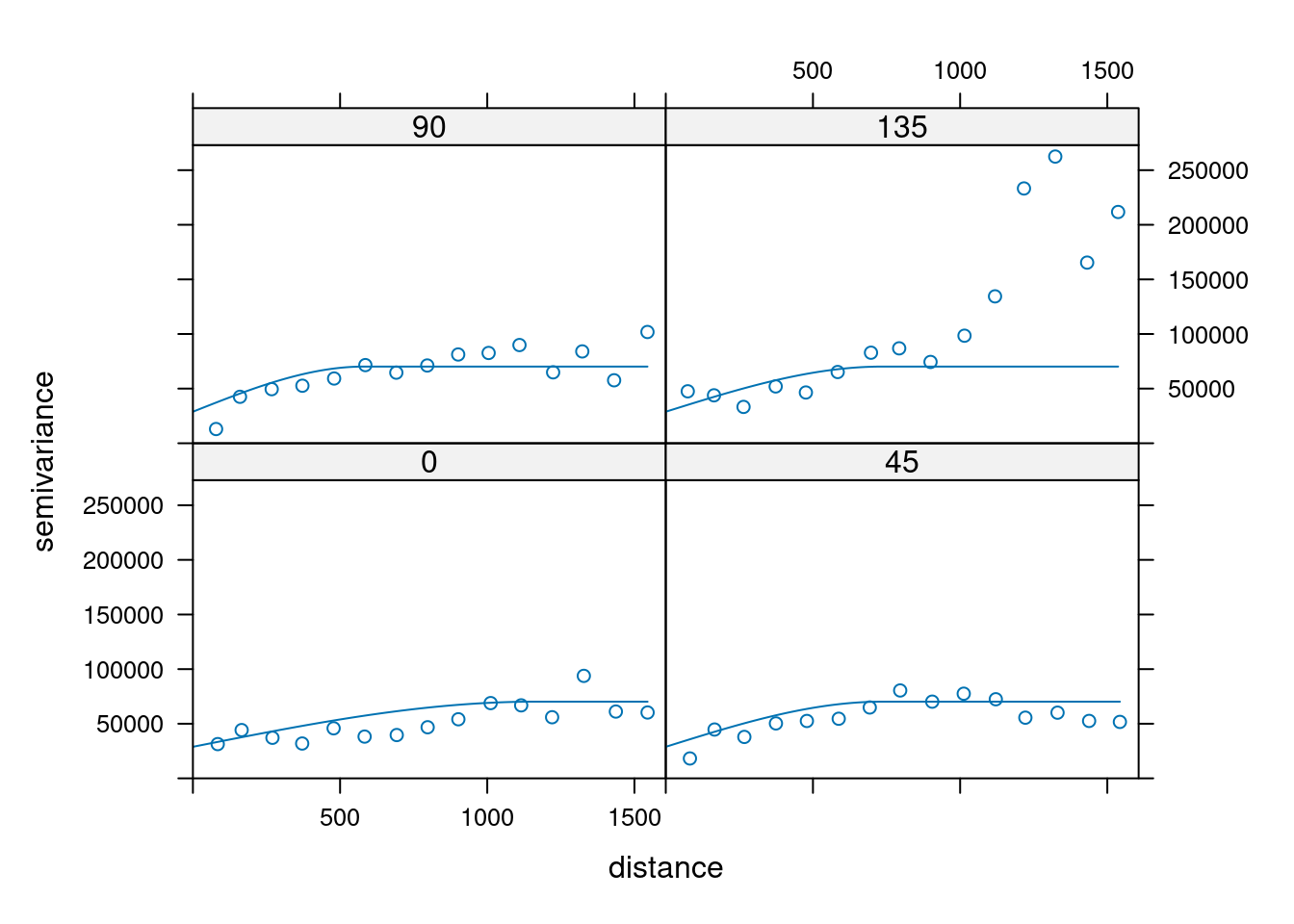
Maybe we need to adjust the angle.
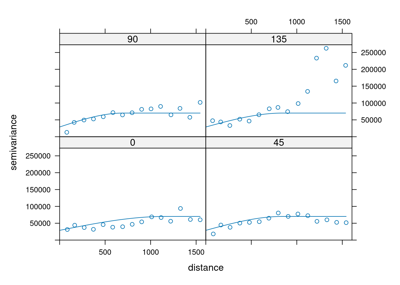
znDist.v <- variogram(zinc ~ I(dist^(1/4)), data= meuse)
znDist.vgmAnis0_05 <- fit.variogram(
                    znDist.v, model=
                      vgm(model="Sph", nugget = NA,
                          anis = c(0,0.5)),
                    fit.ranges=TRUE, fit.sills=TRUE)

plot(zn.vDist.dir, znDist.vgmAnis0_05)
Try to fine tune some parameters:
znDist.vgmAnis0_06 <- fit.variogram(
                    znDist.v, model=
                      vgm(model="Sph", nugget = NA,
                          anis = c(0,0.6)),
                    fit.ranges=TRUE, fit.sills=TRUE)

plot(zn.vDist.dir, znDist.vgmAnis0_06)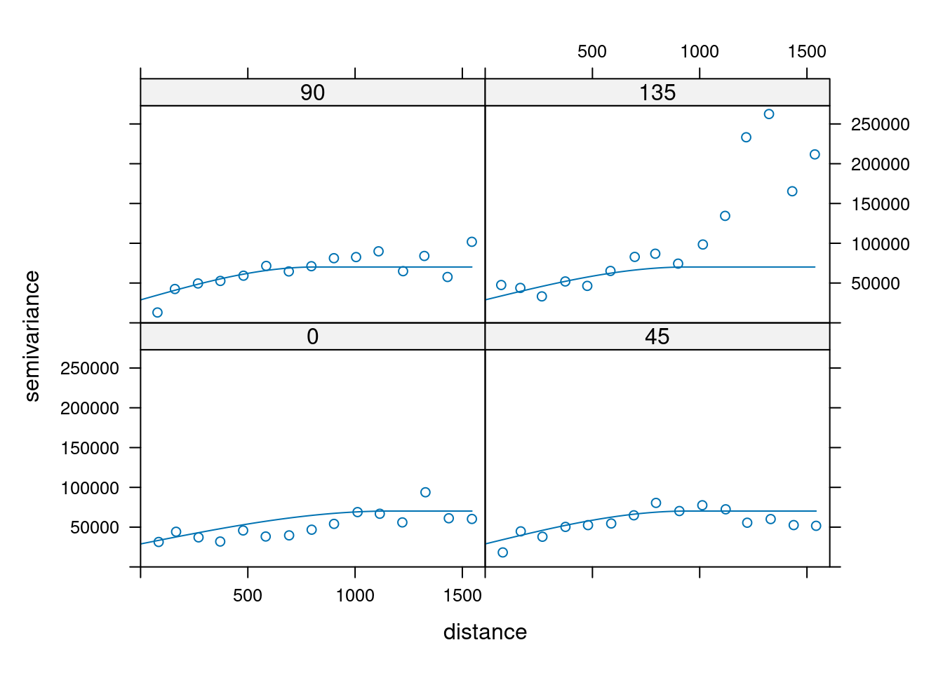
znDist.vgmAnis0_04 <- fit.variogram(
                    znDist.v, model=
                      vgm(model="Sph", nugget = NA,
                          anis = c(0,0.4)),
                    fit.ranges=TRUE, fit.sills=TRUE)

plot(zn.vDist.dir, znDist.vgmAnis0_04)
znDist.vgmAnis0_07 <- fit.variogram(
                    znDist.v, model=
                      vgm(model="Sph", nugget = NA,
                          anis = c(0,0.7)),
                    fit.ranges=TRUE, fit.sills=TRUE)

plot(zn.vDist.dir, znDist.vgmAnis0_07)
znDist.anis0_04.cv <- krige.cv(zinc ~ I(dist^(1/4)),
                      locations = meuse,
                      model =  znDist.vgmAnis0_04, nfold=5)
znDist.anis0_05.cv <- krige.cv(zinc ~ I(dist^(1/4)),
                      locations = meuse,
                      model =  znDist.vgmAnis0_05, nfold=5)
znDist.anis0_06.cv <- krige.cv(zinc ~ I(dist^(1/4)),
                      locations = meuse,
                      model =  znDist.vgmAnis0_06, nfold=5)
znDist.anis0_07.cv <- krige.cv(zinc ~ I(dist^(1/4)),
                      locations = meuse,
                      model =  znDist.vgmAnis0_07, nfold=5)


sqrt(mean(znDist.anis0_04.cv$residual^2))
## [1] 220.5327## [1] 230.8421## [1] 219.7862## [1] 219.6226In a real world setting, we could use e.g. optim to optimize the parameters by crossvalidation. But we leave it for now and use the best model for prediction.
predZincDist <- krige(zinc ~ I(dist^(1/4)),
                    locations = meuse,
                    newdata = meuse.grid, model =  znDist.vgmAnis0_07)
## [using universal kriging]tm_shape(subset(predZincDistRas, subset = "var1.pred")) +
tm_raster(col="var1.pred", title = "Prediction [ppm]", n=9,
legend.reverse = TRUE, palette = "Reds") +
tm_shape(meuse_sf) +
tm_bubbles(size="zinc", alpha=0.5) +
tm_scale_bar() +
tm_layout(title = "Zinc, fourth root of distance to river",
legend.outside = TRUE, attr.outside = TRUE)## ## ── tmap v3 code detected ───────────────────────────────────────────────────────## [v3->v4] `tm_tm_raster()`: migrate the argument(s) related to the scale of the
## visual variable `col` namely 'n', 'palette' (rename to 'values') to col.scale =
## tm_scale(<HERE>).
## [v3->v4] `tm_raster()`: migrate the argument(s) related to the legend of the
## visual variable `col` namely 'title', 'legend.reverse' (rename to 'reverse') to
## 'col.legend = tm_legend(<HERE>)'
## [v3->v4] `tm_bubbles()`: use `fill_alpha` instead of `alpha`.
## ! `tm_scale_bar()` is deprecated. Please use `tm_scalebar()` instead.
## [v3->v4] `tm_layout()`: use `tm_title()` instead of `tm_layout(title = )`
## [cols4all] color palettes: use palettes from the R package cols4all. Run
## `cols4all::c4a_gui()` to explore them. The old palette name "Reds" is named
## "brewer.reds"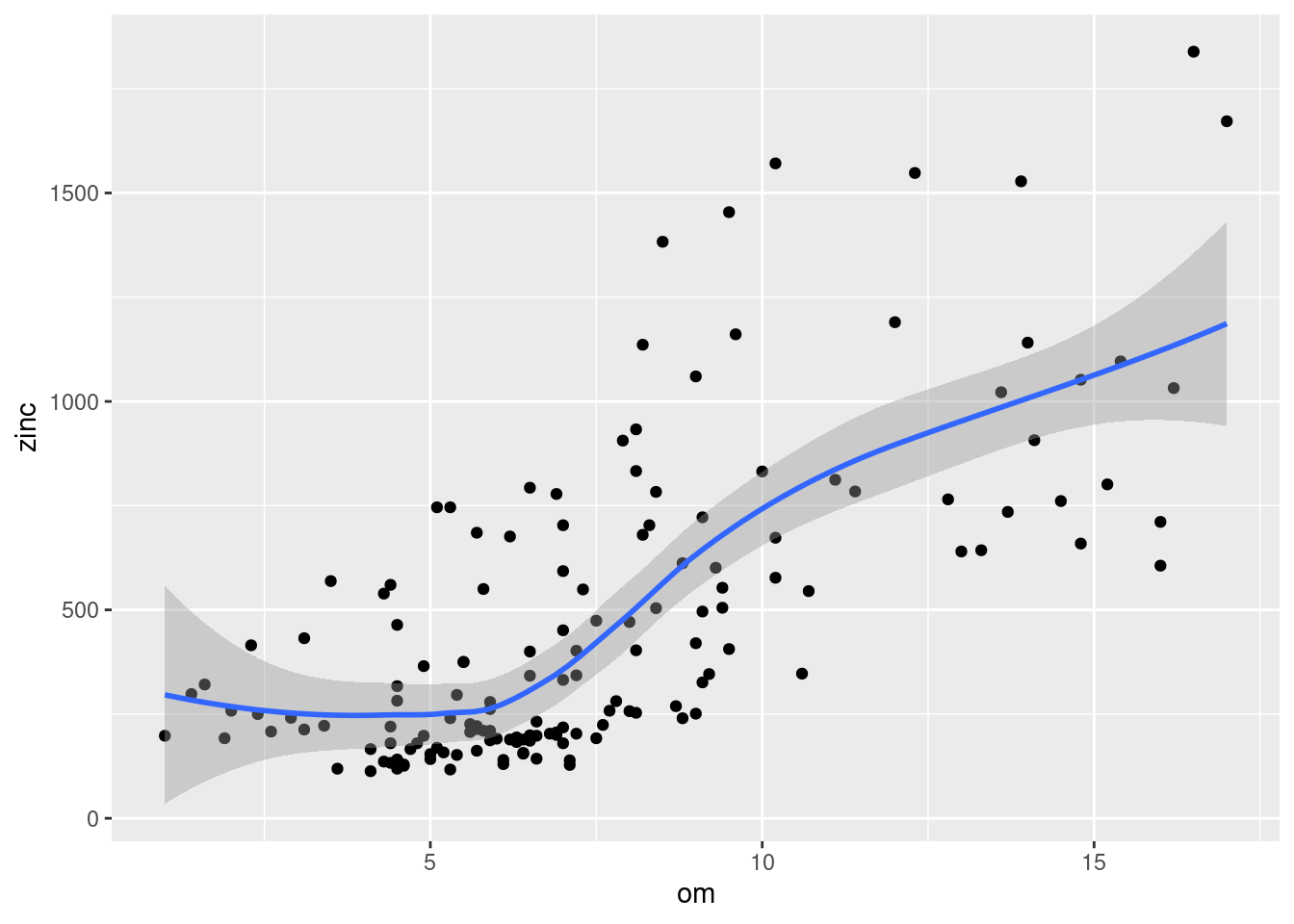
For the standard error we need to take the square root of the prediction variance.
tm_shape(subset(predZincDistRas, subset = "var1.var") %>% sqrt()) +
  tm_raster(col="layer", title = "Standard error [ppm]", n=9, palette = "Purples") +
  tm_shape(meuse_sf) +
  tm_bubbles(size="zinc", alpha=0.5) +
  tm_scale_bar() +
  tm_layout(title = "Zinc, fourth root of distance to river",
            legend.outside = TRUE, attr.outside = TRUE)
## ## ── tmap v3 code detected ───────────────────────────────────────────────────────## [v3->v4] `tm_tm_raster()`: migrate the argument(s) related to the scale of the
## visual variable `col` namely 'n', 'palette' (rename to 'values') to col.scale =
## tm_scale(<HERE>).
## [v3->v4] `tm_raster()`: migrate the argument(s) related to the legend of the
## visual variable `col` namely 'title' to 'col.legend = tm_legend(<HERE>)'
## [v3->v4] `tm_bubbles()`: use `fill_alpha` instead of `alpha`.
## ! `tm_scale_bar()` is deprecated. Please use `tm_scalebar()` instead.
## [v3->v4] `tm_layout()`: use `tm_title()` instead of `tm_layout(title = )`
## [cols4all] color palettes: use palettes from the R package cols4all. Run
## `cols4all::c4a_gui()` to explore them. The old palette name "Purples" is named
## "brewer.purples"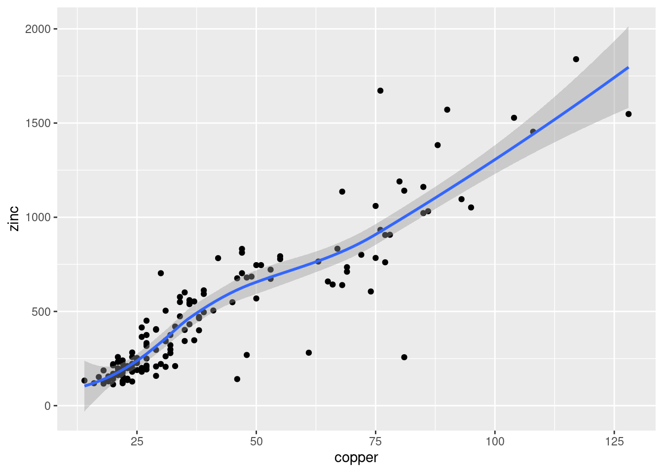
14.5.2 Cokriging
Let’s investigate some relationship between zinc and organic matter as well as with other heavy metals.
## `geom_smooth()` using method = 'loess' and formula = 'y ~ x'## Warning: Removed 2 rows containing non-finite outside the scale range
## (`stat_smooth()`).## Warning: Removed 2 rows containing missing values or values outside the scale range
## (`geom_point()`).
## `geom_smooth()` using method = 'loess' and formula = 'y ~ x'
##              zinc        om    copper   cadmium      lead
## zinc    1.0000000 0.6842578 0.9082695 0.9162139 0.9546913
## om      0.6842578 1.0000000 0.7347169 0.7307845 0.5535007
## copper  0.9082695 0.7347169 1.0000000 0.9254499 0.8183069
## cadmium 0.9162139 0.7307845 0.9254499 1.0000000 0.7989466
## lead    0.9546913 0.5535007 0.8183069 0.7989466 1.0000000
For a multivariate analysis we need with staring organizing information. In the follwoing we collect the two variables we are interestd in in an gstat object, that is created by the function of the same name. We start with just two variables: zincand copper.
g <- gstat(NULL, "zinc", zinc ~ I(dist^(1/4)), data = meuse) # create new gstat object
g <- gstat(g, "copper", copper ~ I(dist^(1/4)), data = meuse) # add to existing gstat object
g
## data:
## zinc : formula = zinc`~`I(dist^(1/4)) ; data dim = 155 x 12
## copper : formula = copper`~`I(dist^(1/4)) ; data dim = 155 x 12Next we create the empirical multivariable variogram and fit a linear model of coregionalization by meany of fit.lmc. The function performs in two steps: first, each variogram model is fitted to a direct or cross variogram. Next each of the partial sill coefficient matrices is approached by its in least squares sense closest positive definite matrices (by setting any negative eigenvalues to zero).
cokrigVm <- variogram(g)
cokrigVmFit <- fit.lmc(cokrigVm, g,
model = vgm("Sph"), fit.ranges = TRUE)
plot(cokrigVm, cokrigVmFit)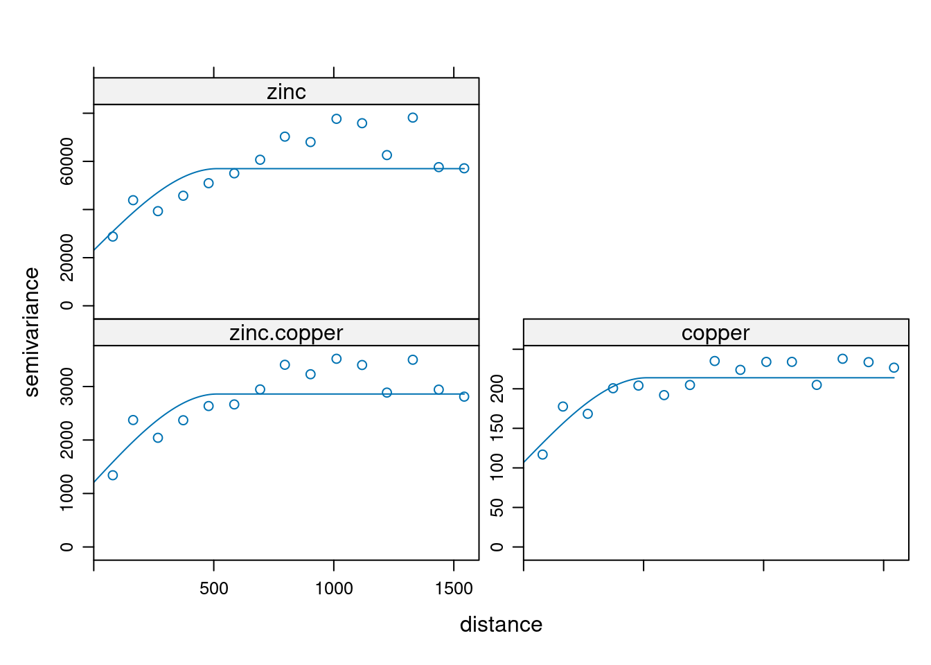
## data:
## zinc : formula = zinc`~`I(dist^(1/4)) ; data dim = 155 x 12
## copper : formula = copper`~`I(dist^(1/4)) ; data dim = 155 x 12
## variograms:
## model psill range
## zinc[1] Nug 28855.17173 0.0000
## zinc[2] Sph 41333.88360 1161.6026
## copper[1] Nug 94.11766 0.0000
## copper[2] Sph 113.60716 404.3957
## zinc.copper[1] Nug 1473.47604 0.0000
## zinc.copper[2] Sph 1750.42613 930.8222The linear model of coregionalization consists here of three models with two components (nugget model and spherical model). While the absoulte semivariance values are very different, the ranges are very similar. The fitted theoretical variograms describes the empirical variogams and the cross variogram quite well. The same shape of the empirical variograms and the cross variogram indicates strong correlation (as spotted before) - if the two variables were not collocated (all variables measured at all locations), the variograms would be helpful even if the correlation analysis would suffer from s small subset for which both varibles were collocated.
For prediction, we actually need a model with identical model components (here nugget and range for the spherical model, the partial sill can vary).
cokrigVmFit <- fit.lmc(cokrigVm, g,
                       model = vgm(psill=1, model="Sph", range=NA, nugget=NA))
plot(cokrigVm, cokrigVmFit)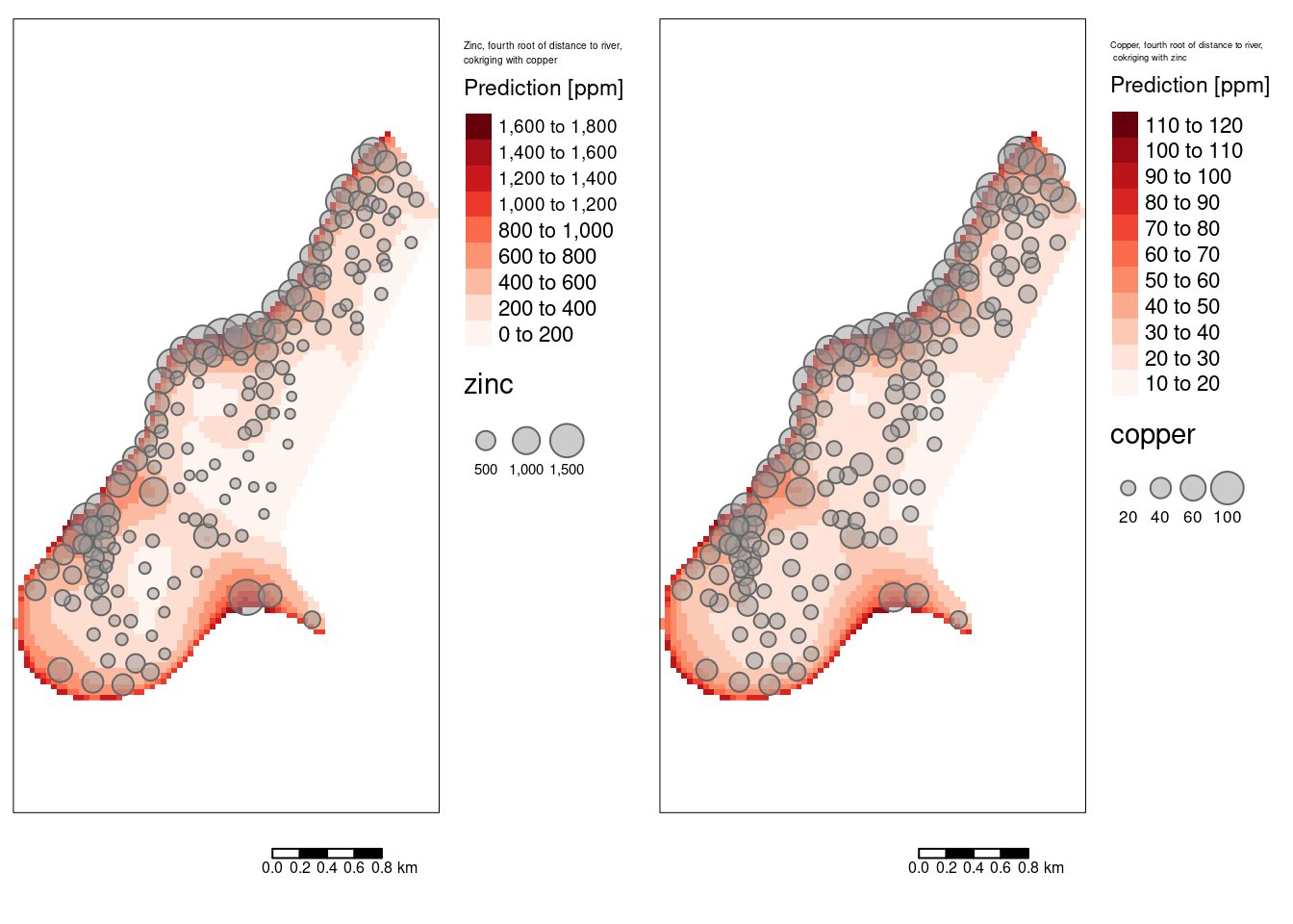
## data:
## zinc : formula = zinc`~`I(dist^(1/4)) ; data dim = 155 x 12
## copper : formula = copper`~`I(dist^(1/4)) ; data dim = 155 x 12
## variograms:
##                model      psill    range
## zinc[1]          Nug 23092.2990   0.0000
## zinc[2]          Sph 33885.4795 514.4008
## copper[1]        Nug   106.8253   0.0000
## copper[2]        Sph   107.1458 514.4008
## zinc.copper[1]   Nug  1208.2791   0.0000
## zinc.copper[2]   Sph  1652.2930 514.4008
Let’s predict (here using predict, which only requires the model and the newdata).
## Linear Model of Coregionalization found. Good.
## [using universal cokriging]m1 <- tm_shape(subset(coKrigeZnCoRas, subset = "zinc.pred")) +
tm_raster(col="zinc.pred", title = "Prediction [ppm]", n=9,
legend.reverse = TRUE, palette = "Reds") +
tm_shape(meuse_sf) +
tm_bubbles(size="zinc", alpha=0.5) +
tm_scale_bar() +
tm_layout(title = "Zinc, fourth root of distance to river,\ncokriging with copper",
legend.outside = TRUE, attr.outside = TRUE)## ## ── tmap v3 code detected ───────────────────────────────────────────────────────## [v3->v4] `tm_tm_raster()`: migrate the argument(s) related to the scale of the
## visual variable `col` namely 'n', 'palette' (rename to 'values') to col.scale =
## tm_scale(<HERE>).
## [v3->v4] `tm_raster()`: migrate the argument(s) related to the legend of the
## visual variable `col` namely 'title', 'legend.reverse' (rename to 'reverse') to
## 'col.legend = tm_legend(<HERE>)'
## [v3->v4] `tm_bubbles()`: use `fill_alpha` instead of `alpha`.
## ! `tm_scale_bar()` is deprecated. Please use `tm_scalebar()` instead.
## [v3->v4] `tm_layout()`: use `tm_title()` instead of `tm_layout(title = )`m2 <- tm_shape(subset(coKrigeZnCoRas, subset = "copper.pred")) +
tm_raster(col="copper.pred", title = "Prediction [ppm]", n=9,
legend.reverse = TRUE, palette = "Reds") +
tm_shape(meuse_sf) +
tm_bubbles(size="copper", alpha=0.5) +
tm_scale_bar() +
tm_layout(title = "Copper, fourth root of distance to river,\n cokriging with zinc",
legend.outside = TRUE, attr.outside = TRUE)## [v3->v4] `tm_raster()`: migrate the argument(s) related to the legend of the
## visual variable `col` namely 'title', 'legend.reverse' (rename to 'reverse') to
## 'col.legend = tm_legend(<HERE>)'
## [v3->v4] `tm_bubbles()`: use `fill_alpha` instead of `alpha`.
## ! `tm_scale_bar()` is deprecated. Please use `tm_scalebar()` instead.
## [v3->v4] `tm_layout()`: use `tm_title()` instead of `tm_layout(title = )`## [cols4all] color palettes: use palettes from the R package cols4all. Run
## `cols4all::c4a_gui()` to explore them. The old palette name "Reds" is named
## "brewer.reds"
## [plot mode] fit legend/component: Some legend items or map compoments do not
## fit well, and are therefore rescaled.
## ℹ Set the tmap option `component.autoscale = FALSE` to disable rescaling.
## [cols4all] color palettes: use palettes from the R package cols4all. Run
## `cols4all::c4a_gui()` to explore them. The old palette name "Reds" is named
## "brewer.reds"
## [plot mode] fit legend/component: Some legend items or map compoments do not
## fit well, and are therefore rescaled.
## ℹ Set the tmap option `component.autoscale = FALSE` to disable rescaling.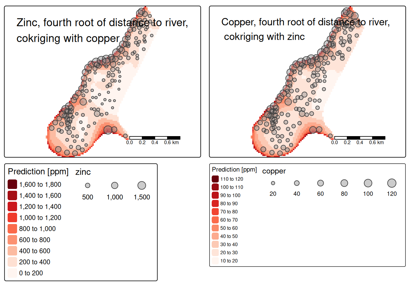
Standard error maps.
m1 <- tm_shape(subset(coKrigeZnCoRas, subset = "zinc.var") %>% sqrt()) +
  tm_raster(col="layer", title = "Standard error [ppm]", n=9, palette = "Purples") +
  tm_shape(meuse_sf) +
  tm_bubbles(size="zinc", alpha=0.5) +
  tm_scale_bar() +
  tm_layout(title = "Zinc,\nfourth root of distance to river,\ncokriging with copper",
            legend.outside = TRUE, attr.outside = TRUE)
## ## ── tmap v3 code detected ───────────────────────────────────────────────────────## [v3->v4] `tm_tm_raster()`: migrate the argument(s) related to the scale of the
## visual variable `col` namely 'n', 'palette' (rename to 'values') to col.scale =
## tm_scale(<HERE>).
## [v3->v4] `tm_raster()`: migrate the argument(s) related to the legend of the
## visual variable `col` namely 'title' to 'col.legend = tm_legend(<HERE>)'
## [v3->v4] `tm_bubbles()`: use `fill_alpha` instead of `alpha`.
## ! `tm_scale_bar()` is deprecated. Please use `tm_scalebar()` instead.
## [v3->v4] `tm_layout()`: use `tm_title()` instead of `tm_layout(title = )`m2 <- tm_shape(subset(coKrigeZnCoRas, subset = "copper.var") %>% sqrt()) +
tm_raster(col="layer", title = "Standard error [ppm]", n=9, palette = "Purples") +
tm_shape(meuse_sf) +
tm_bubbles(size="copper", alpha=0.5) +
tm_scale_bar() +
tm_layout(title = "Copper, \nfourth root of distance to river,\ncokriging with zinc",
legend.outside = TRUE, attr.outside = TRUE)## [v3->v4] `tm_raster()`: migrate the argument(s) related to the legend of the
## visual variable `col` namely 'title' to 'col.legend = tm_legend(<HERE>)'
## [v3->v4] `tm_bubbles()`: use `fill_alpha` instead of `alpha`.
## ! `tm_scale_bar()` is deprecated. Please use `tm_scalebar()` instead.
## [v3->v4] `tm_layout()`: use `tm_title()` instead of `tm_layout(title = )`m3 <- tm_shape(subset(coKrigeZnCoRas, subset = "cov.zinc.copper") ) +
tm_raster(col="cov.zinc.copper", title = "Covariance zinc-copper", n=9, palette = "Purples") +
tm_scale_bar() +
tm_layout(title = "Copper and zinc,\nfourth root of distance to river,\ncokriging",
legend.outside = TRUE, attr.outside = TRUE)## [v3->v4] `tm_raster()`: migrate the argument(s) related to the legend of the
## visual variable `col` namely 'title' to 'col.legend = tm_legend(<HERE>)'
## ! `tm_scale_bar()` is deprecated. Please use `tm_scalebar()` instead.
## [v3->v4] `tm_layout()`: use `tm_title()` instead of `tm_layout(title = )`## [cols4all] color palettes: use palettes from the R package cols4all. Run
## `cols4all::c4a_gui()` to explore them. The old palette name "Purples" is named
## "brewer.purples"
## [plot mode] fit legend/component: Some legend items or map compoments do not
## fit well, and are therefore rescaled.
## ℹ Set the tmap option `component.autoscale = FALSE` to disable rescaling.
## [cols4all] color palettes: use palettes from the R package cols4all. Run
## `cols4all::c4a_gui()` to explore them. The old palette name "Purples" is named
## "brewer.purples"
## [plot mode] fit legend/component: Some legend items or map compoments do not
## fit well, and are therefore rescaled.
## ℹ Set the tmap option `component.autoscale = FALSE` to disable rescaling.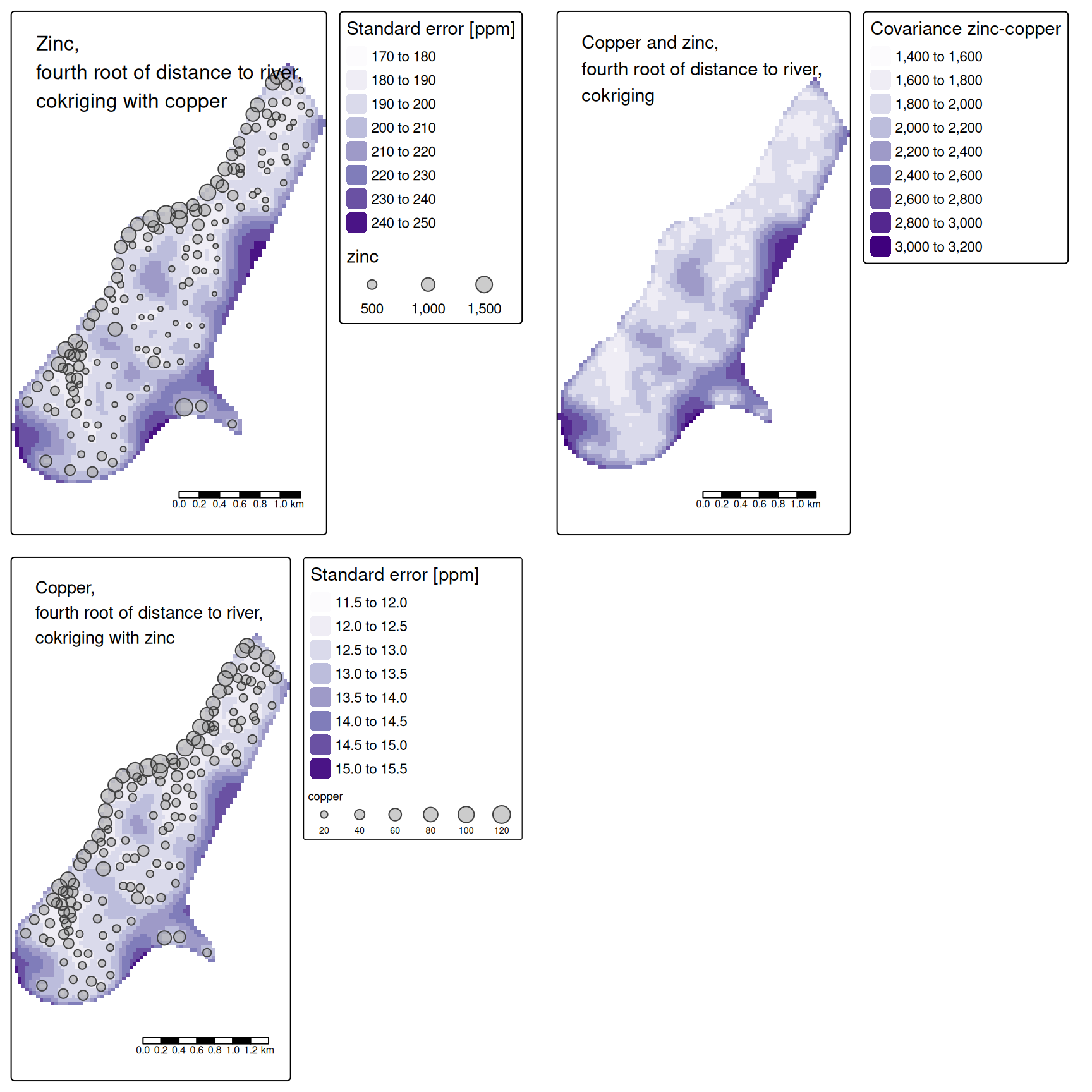
Is the cokriging model better than the normal one? (Ignoring anisotropy for now). Specifying remove.all = FALSE implies that during cross-validation only the primary variable is dropped (zinc) while copper is keept in the model. This simulates the case of non collocated variables. Given the high correlation between zinc and copper this is for sure and advantage of the model.
## Linear Model of Coregionalization found. Good.
## [using universal cokriging]
## Linear Model of Coregionalization found. Good.
## [using universal cokriging]
## Linear Model of Coregionalization found. Good.
## [using universal cokriging]
## Linear Model of Coregionalization found. Good.
## [using universal cokriging]
## Linear Model of Coregionalization found. Good.
## [using universal cokriging]
Residuals are calculated for the first variable (here zinc).
## [1] 137.639What if we perform a cross-validation there both variables are dropped for the test?
## Linear Model of Coregionalization found. Good.
## [using universal cokriging]
## Linear Model of Coregionalization found. Good.
## [using universal cokriging]
## Linear Model of Coregionalization found. Good.
## [using universal cokriging]
## Linear Model of Coregionalization found. Good.
## [using universal cokriging]
## Linear Model of Coregionalization found. Good.
## [using universal cokriging]## [1] 223.7429How does that compare with the isotropic universal kriging model for zinc?
#znDist.v <- variogram(zinc ~ I(dist^(1/4)), data= meuse)
znDist.vgm <- fit.variogram(
                    znDist.v, model=
                      vgm(model="Sph", nugget = NA))
g.znDist <- gstat(NULL, id="zinc",formula = zinc ~ I(dist^(1/4)), model= znDist.vgm, data= meuse)
g.znDist.cv <- gstat.cv(g.znDist, nfold = 5)
## [using universal kriging]
## [using universal kriging]
## [using universal kriging]
## [using universal kriging]
## [using universal kriging]## [1] 219.2117We see that the cokriging model performed a bit better. However, we should for a real wolrd test run the cross-validation repeated times (see above).
References
At the time of writing installation is a bit tricky as there are some issued triggered by the required package
RandomFields. However, downloading newest archived versions and installing from sources should do the trick.↩︎As long as we use global kriging that uses all available observations. If we would use local kriging, there only the closest k-neighbors or all neighbors in a search distance are used for the interpolation, \(C\) and thereby \(C^{-1}\) would change as well.↩︎