Chapter 12 Spatial regression analysis - spatial eigenvector mapping
library(knitr)
library(rmdformats)
require(sf)
require(spdep)
require(ggpubr)
require(spatialreg)
require(ggplot2)
require(tidyverse)
require(tmap)
require(GGally)
set.seed(42)
12.1 Cheat sheet
The functions for spatial eigenvector mapping are provided by the package {spatialreg}
ME- uses a brute force approach to select the eigenvectorsfittedis used to extract the selected eigenvectors from the object returned byME
12.2 Theory
12.2.1 Spatial eigenvector mapping
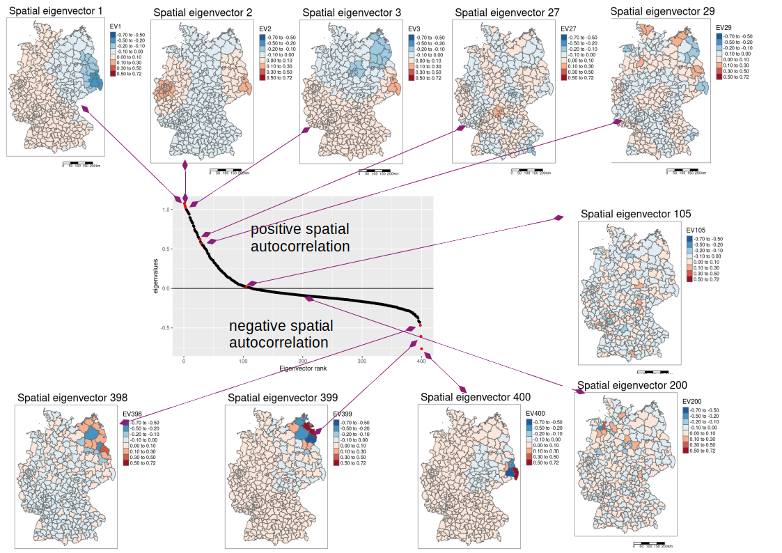
The idea behind the spatial eigenvector mapping approach (Griffith et al., 2019) is to use additional covariates that absorb the spatial autocorrelation, leading to unbiased estimators for the other predictors. The additional covariates are based on the eigenfunction decomposition of the spatial weight matrix \(W\). Eigenvectors of \(W\) represent the decompositions the spatial weight Matrix into all mutually orthogonal eigenvectors. \(W\) represents all possibilities how spatial autocorrelation could be involved given the neighborhood definition and the weighting. The eigenvector decomposition separates that information into orthogonal (i.e. independent) components - this is similar to the principal component analysis. The dimension of the (quadratic) weight matrix \(W\) is defined by the number of spatial units. The eigenvector composition leads to the same number of spatial eigenvectors. If we have 400 spatial units this leads to 400 spatial eigenvectors.
Those spatial eigenvectors with positive eigenvalues represent positive autocorrelation, whereas eigenvectors with negative eigenvalues represent negative autocorrelation. The higher the eigenvalue of an eigenvector the longer ranging the spatial autocorrelation structure. Typically, the eigenvectors are sorted by their eigenvalue from the largest to the smallest. This can bee seen in the following figure: the maps of the eigenvecotrs 1 to 3 show long ranging gradients while the eigenvectors 27 and 29 are examples of shorter range spatial autocorrelation. Eigenvector 105 and eigenvector 200 show non significant spatial autocorrelation while the eigenvectors 398 till 400 show very short ranged negative spatial autocorrelation.
(#fig:fig:gwr)Geographically weighted regression
The corresponding Moran’s I values for the shown spatial eigenvectors are as follows:
- EV1: 0.95
- EV2: 0.99
- EV3: 0.96
- …
- EV27: 0.61
- …
- EV29: 0.56
- …
- EV105: 0.02
- …
- EV200: -0.09
- …
- EV398: -0.44
- EV399: -0.47
- EV400: -0.51
To be more precise, the eigenvector decomposition is not based on the raw matrix \(W\) but on the following transformation:
\[ M * W * M \] there
- \(n\) x \(n\) is the dimension of the quadratic matrix \(W\)
- $ M = (I - 1 1^T/n)$ is a quadratic projection matrix of dimension \(n\) x \(n\)
- \(I\) is the identity matrix of dimension \(n\) x \(n\), i.e. a matrix with 1 at the diagonal and 0 everywhere else
- \(1\) is a matrix of dimension \(n\) x \(1\) with all elements being 1
- \(*\) is the matrix multiplication operator (as opposed to the scalar multiplication)
The eigenvectors are mutually orthogonal and uncorrelated (Griffith, 2000): the symmetry of matrix \(W\) ensures orthogonality, and the projection matrix $ M = (I - 1 1^T/n)$ ensures that eigenvectors have zero means, guaranteeing uncorrelatedness. That is, \(E_i * E_i^T = I\) and \(E^T * 1 = 0\), and the correlation between any pair of eigenvectors \(E_i\) and \(E_j\), is zero when \(i \neq j\). The eigenvectors portray distinct, selected map patterns. Each eigenvector portrays a different map pattern exhibiting a specified level of spatial autocorrelation when it is mapped onto the \(n\) areal units associated with the corresponding spatial weights matrix \(W\) (Tiefelsdorf and Boots, 1995). They also establish that the Moran coefficient (MC) value for a mapped eigenvector is equal to a function of its corresponding eigenvalue (i.e., \(MC_j = \frac{n}{1^TW1⋅\lambda_j}\), for \(E_j\)). Given a spatial weights matrix \(W\), the feasible range of MC values is determined by the largest and smallest eigenvalues; i.e., by \(\lambda_1\) and \(\lambda_n\) (De Jong et al., 1984).
12.2.2 Selection of eigenvectors
The questions is now, which of the spatial eigenvectors should be included in the regression model. The idea is to keep the predictors selected previously as fixed and add the spatial eigenvectors one by one. If one is significant and reduces the spatial autocorreltaion it is kept in the model and we continue with the next eigenvector. We only incorporate the spatial eigenvectors with positive eigenvalues. Often a further pre-selection is performed by testing only the eigenvectors there the eigenvalue is above a threshold. Testing of eigenvectors is done based on the order of the eigenvalues.
The function ME uses brute force eigenvector selection to reach a subset of such vectors to be added to the RHS of the GLM model to reduce residual autocorrelation to below the specified alpha value (defaults to 0.05). Since eigenvector selection only works on symmetric weights, the weights are made symmetric beforehand.
12.3 Case study
## Reading layer `kreiseWithCovidMeldeWeeklyCleaned' from data source
##   `/home/slautenbach/Documents/lehre/HD/git_areas/spatial_data_science/spatial-data-science/data/covidKreise.gpkg'
##   using driver `GPKG'
## Simple feature collection with 400 features and 145 fields
## Geometry type: MULTIPOLYGON
## Dimension:     XY
## Bounding box:  xmin: 280371.1 ymin: 5235856 xmax: 921292.4 ymax: 6101444
## Projected CRS: ETRS89 / UTM zone 32N## Warning: st_point_on_surface assumes attributes are constant over geometriesdistnb <- dnearneigh(poSurfKreise, d1=1, d2= 70*10^3)
unionedNb <- union.nb(distnb, polynb)
dlist <- nbdists(unionedNb, st_coordinates(poSurfKreise))
dlist <- lapply(dlist, function(x) 1/x)
unionedListw_d <- nb2listw(unionedNb, glist=dlist, style = "W")12.3.1 Spatial eigenvector selection
We use the quasipoisson model here as it can be easily used with ME. For the negative binomial we would need to perform the spatial eigenvector mapping by writing our own code that is not too complex but out of hands for our purpose here.
We use ME: the function gets the formula object that defines our current model (for which we detected spatial autocorrelation in the residuals). We can define the family and the offset as in glm and need to provide the spatial weight matrix \(W\) by means of the weightes list.
meQp <- spatialreg::ME(sumCasesTotal ~ Stimmenanteile.AfD + Auslaenderanteil +
                         Hochqualifizierte + Langzeitarbeitslosenquote +
                         Einpendler + Studierende,
                       family = quasipoisson,
                       data = covidKreise,
                       offset = log(EWZ), listw = unionedListw_d)
Refitting GLM under incorporation of the selected spatial eigenvectors. The selected spatial eigenvectors are added by fitted(meQp).
modelSevmQp <- glm(sumCasesTotal ~ Stimmenanteile.AfD + Auslaenderanteil +
                         Hochqualifizierte + Langzeitarbeitslosenquote +
                         Einpendler + Studierende + fitted(meQp),
                   family = quasipoisson,
                   data = covidKreise,
                   offset = log(EWZ))
summary(modelSevmQp)
##
## Call:
## glm(formula = sumCasesTotal ~ Stimmenanteile.AfD + Auslaenderanteil +
## Hochqualifizierte + Langzeitarbeitslosenquote + Einpendler +
## Studierende + fitted(meQp), family = quasipoisson, data = covidKreise,
## offset = log(EWZ))
##
## Coefficients:
## Estimate Std. Error t value Pr(>|t|)
## (Intercept) -1.3071964 0.0401106 -32.590 < 2e-16 ***
## Stimmenanteile.AfD 0.0188688 0.0009921 19.019 < 2e-16 ***
## Auslaenderanteil 0.0088407 0.0011785 7.502 4.35e-13 ***
## Hochqualifizierte -0.0027657 0.0011286 -2.450 0.014709 *
## Langzeitarbeitslosenquote -0.0573016 0.0035142 -16.306 < 2e-16 ***
## Einpendler -0.0011573 0.0004290 -2.698 0.007291 **
## Studierende 0.0001983 0.0001174 1.689 0.091968 .
## fitted(meQp)vec4 -0.9226405 0.0910536 -10.133 < 2e-16 ***
## fitted(meQp)vec21 -0.5556732 0.1007379 -5.516 6.35e-08 ***
## fitted(meQp)vec20 -0.5574915 0.0962049 -5.795 1.42e-08 ***
## fitted(meQp)vec6 0.2185211 0.0981631 2.226 0.026583 *
## fitted(meQp)vec26 -0.2825856 0.0975831 -2.896 0.003996 **
## fitted(meQp)vec22 -0.2967855 0.0886427 -3.348 0.000893 ***
## ---
## Signif. codes: 0 '***' 0.001 '**' 0.01 '*' 0.05 '.' 0.1 ' ' 1
##
## (Dispersion parameter for quasipoisson family taken to be 478.5901)
##
## Null deviance: 555100 on 399 degrees of freedom
## Residual deviance: 184879 on 387 degrees of freedom
## AIC: NA
##
## Number of Fisher Scoring iterations: 4The procedure added 6 spatial eigenvectors to the model. Together this leads to a more than satisfying amount of explained deviance. However, we need to keep in mind that a good share of that come from the spatial eigenvectors.
## [1] 0.666945212.3.2 Model selection
The share of students now became insignificant so we might want to drop the predictor from the model. It is good practice to reselect the spatial eigenvectors if the drop or add a predictor.
meQp <- spatialreg::ME(sumCasesTotal ~ Stimmenanteile.AfD + Auslaenderanteil +
    Hochqualifizierte + Langzeitarbeitslosenquote + Einpendler,
                       family = quasipoisson,
                       data = covidKreise,
                       offset = log(EWZ),
                       listw = unionedListw_d)
Refitting GLM under incorporation of the selected spatial eigenvectors:
modelSevmQp <- glm(sumCasesTotal ~ Stimmenanteile.AfD + Auslaenderanteil +
    Hochqualifizierte + Langzeitarbeitslosenquote + Einpendler  + fitted(meQp),
                   family = quasipoisson, offset = log(EWZ),
                   data = covidKreise)
summary(modelSevmQp)
##
## Call:
## glm(formula = sumCasesTotal ~ Stimmenanteile.AfD + Auslaenderanteil +
## Hochqualifizierte + Langzeitarbeitslosenquote + Einpendler +
## fitted(meQp), family = quasipoisson, data = covidKreise,
## offset = log(EWZ))
##
## Coefficients:
## Estimate Std. Error t value Pr(>|t|)
## (Intercept) -1.2916940 0.0395103 -32.693 < 2e-16 ***
## Stimmenanteile.AfD 0.0185317 0.0009606 19.292 < 2e-16 ***
## Auslaenderanteil 0.0096656 0.0011720 8.247 2.56e-15 ***
## Hochqualifizierte -0.0020848 0.0010039 -2.077 0.038489 *
## Langzeitarbeitslosenquote -0.0577396 0.0034061 -16.952 < 2e-16 ***
## Einpendler -0.0014843 0.0004265 -3.480 0.000559 ***
## fitted(meQp)vec4 -0.8582883 0.0902518 -9.510 < 2e-16 ***
## fitted(meQp)vec21 -0.5489610 0.0989308 -5.549 5.34e-08 ***
## fitted(meQp)vec20 -0.5465377 0.0939012 -5.820 1.23e-08 ***
## fitted(meQp)vec6 0.2242360 0.0960668 2.334 0.020098 *
## fitted(meQp)vec26 -0.2879102 0.0954718 -3.016 0.002733 **
## fitted(meQp)vec22 -0.3063519 0.0867027 -3.533 0.000460 ***
## fitted(meQp)vec13 0.3795482 0.0890986 4.260 2.57e-05 ***
## ---
## Signif. codes: 0 '***' 0.001 '**' 0.01 '*' 0.05 '.' 0.1 ' ' 1
##
## (Dispersion parameter for quasipoisson family taken to be 459.1879)
##
## Null deviance: 555100 on 399 degrees of freedom
## Residual deviance: 177917 on 387 degrees of freedom
## AIC: NA
##
## Number of Fisher Scoring iterations: 4The eigenvectors selected did not change then we dropped the predictor - however, this is not always the case.
As the predictor for the share of the highly qualified workers is marginally significantly different from zero we could also drop it. However, we keep it here in the model.
12.3.3 Plotting selected spatial eigenvectors
Presumably we have missed a lot of other predictors that are now partially absorbed into different eigenvectors. It might be worth to plot and investigate the eigenvectors that made it into the model. Therefore, we attach the selected eigenvectors to the sf object and plot them.
##       vec4                vec21               vec20
##  Min.   :-0.1121802   Min.   :-0.165692   Min.   :-0.13859
##  1st Qu.:-0.0318616   1st Qu.:-0.034497   1st Qu.:-0.03242
##  Median : 0.0004217   Median : 0.003475   Median :-0.00302
##  Mean   : 0.0000000   Mean   : 0.000000   Mean   : 0.00000
##  3rd Qu.: 0.0237315   3rd Qu.: 0.029910   3rd Qu.: 0.03421
##  Max.   : 0.1205038   Max.   : 0.124410   Max.   : 0.13860
##       vec6               vec26               vec22
##  Min.   :-0.182795   Min.   :-0.137955   Min.   :-0.215188
##  1st Qu.:-0.017039   1st Qu.:-0.029115   1st Qu.:-0.022795
##  Median :-0.001011   Median : 0.001045   Median : 0.002359
##  Mean   : 0.000000   Mean   : 0.000000   Mean   : 0.000000
##  3rd Qu.: 0.017834   3rd Qu.: 0.029467   3rd Qu.: 0.021287
##  Max.   : 0.178978   Max.   : 0.119625   Max.   : 0.240824
##      vec13
##  Min.   :-0.143519
##  1st Qu.:-0.022562
##  Median :-0.002557
##  Mean   : 0.000000
##  3rd Qu.: 0.019189
## Max. : 0.180259#theBreaks <- seq(from = min(fitted(meQp)), to = max(fitted(meQp)), length.out= 6)
tm_shape(covidKreiseSvem) +
tm_polygons(col= colnames(sevQp), palette = "-RdBu", lwd=.5,
n = 7, midpoint=0, legend.show = FALSE) +
tm_layout(main.title = "Selected spatial eigenvectors", legend.outside = TRUE,
attr.outside = TRUE, panel.show = TRUE,
panel.labels = colnames(sevQp)) +
tm_scale_bar()## ## ── tmap v3 code detected ───────────────────────────────────────────────────────## [v3->v4] `tm_tm_polygons()`: migrate the argument(s) related to the scale of
## the visual variable `fill` namely 'n', 'midpoint', 'palette' (rename to
## 'values') to fill.scale = tm_scale(<HERE>).
## ℹ For small multiples, specify a 'tm_scale_' for each multiple, and put them in
## a list: 'fill.scale = list(<scale1>, <scale2>, ...)'
## [v3->v4] `tm_polygons()`: use 'fill' for the fill color of polygons/symbols
## (instead of 'col'), and 'col' for the outlines (instead of 'border.col').
## [v3->v4] `tm_polygons()`: use `fill.legend = tm_legend_hide()` instead of
## `legend.show = FALSE`.
## [v3->v4] `tm_layout()`: use `tm_title()` instead of `tm_layout(main.title = )`
## ! `tm_scale_bar()` is deprecated. Please use `tm_scalebar()` instead.
## Multiple palettes called "rd_bu" found: "brewer.rd_bu", "matplotlib.rd_bu". The first one, "brewer.rd_bu", is returned.
##
## [cols4all] color palettes: use palettes from the R package cols4all. Run
## `cols4all::c4a_gui()` to explore them. The old palette name "-RdBu" is named
## "rd_bu" (in long format "brewer.rd_bu")
## Multiple palettes called "rd_bu" found: "brewer.rd_bu", "matplotlib.rd_bu". The first one, "brewer.rd_bu", is returned.
##
## Multiple palettes called "rd_bu" found: "brewer.rd_bu", "matplotlib.rd_bu". The first one, "brewer.rd_bu", is returned.
##
## Multiple palettes called "rd_bu" found: "brewer.rd_bu", "matplotlib.rd_bu". The first one, "brewer.rd_bu", is returned.
##
## Multiple palettes called "rd_bu" found: "brewer.rd_bu", "matplotlib.rd_bu". The first one, "brewer.rd_bu", is returned.
##
## Multiple palettes called "rd_bu" found: "brewer.rd_bu", "matplotlib.rd_bu". The first one, "brewer.rd_bu", is returned.
##
## Multiple palettes called "rd_bu" found: "brewer.rd_bu", "matplotlib.rd_bu". The first one, "brewer.rd_bu", is returned.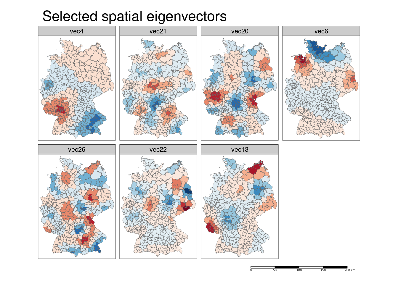
The spatial eigenvectors included in the model capture broadly speaking:
- a contrast between the southern part of Bavaria and Rhineland-Palatina and Saarland and parts of Baden-Württemberg which centers around Mannheim, Ludwigshafen and the Rhein-Neckar district as well as with another cluster in the Ruhrgebiet (eigenvector 4)
- a contrast between Schleswig-Holstein and parts of Mecklenburg Vorpommern and Ostfriesland and Brandenburg (eigenvector 6)
- a contrast between a region around Rostock and a region around Trier on the one side and the regions Berlin and Frankfurt on the other side (eigenvector 13)
- shorter ranged contrasts between Bonn/Rerhin-Sieg/Eifel/Koblenz and Vogtland/Hof and Schweinsfurt/Würzburg and Bitterfeld/Dessau-Roßlau (eigenvector 20)
- …
Note that the legends have not been unified but zero has always been set as the midpoint - i.e. blue always indicates negative values and red positive values. For the interpretation we need to look at the sign of the regression coefficient and the sign of the eigenvector. For eigenvector 4 the sign is negative, that means the model predicts higher incidence rates in Bavaria (blue indicates negative values) and the Ruhrgebiet and lower incidence rates in the Rhein-Neckar region.
The spatial eigenvectors might help us to derive hypothesis about missing covariates that could be incorporated in the model. In any case they absorb a good share of the spatial autocorrelation in the residuals.
Selection of districts with high or low values of a specific eigenvector can be done for example using slice_max or slice_min
st_drop_geometry(covidKreiseSvem) %>%
  slice_max(order_by = vec20, n = 15) %>%
  dplyr::select(GEN, vec20)
## GEN vec20
## 1 Neuwied 0.13860376
## 2 Ahrweiler 0.13562872
## 3 Mayen-Koblenz 0.13323352
## 4 Koblenz 0.12933707
## 5 Hof 0.12670362
## 6 Hof 0.12458526
## 7 Westerwaldkreis 0.12288344
## 8 Wunsiedel i. Fichtelgebirge 0.10908897
## 9 Bonn 0.10867072
## 10 Rhein-Sieg-Kreis 0.10719431
## 11 Altenkirchen (Westerwald) 0.10659562
## 12 Vogtlandkreis 0.10307695
## 13 Rhein-Lahn-Kreis 0.10301496
## 14 Tirschenreuth 0.10012535
## 15 Vulkaneifel 0.09503687st_drop_geometry(covidKreiseSvem) %>%
slice_min(order_by = vec20, n = 20) %>%
dplyr::select(GEN, vec20)## GEN vec20
## 1 Schweinfurt -0.13858896
## 2 Würzburg -0.13304414
## 3 Schweinfurt -0.13127589
## 4 Würzburg -0.12690830
## 5 Bad Kissingen -0.11502402
## 6 Main-Spessart -0.11061198
## 7 Anhalt-Bitterfeld -0.10729847
## 8 Kitzingen -0.10277726
## 9 Dessau-Roßlau -0.09812303
## 10 Salzlandkreis -0.09345552
## 11 Rhön-Grabfeld -0.08992219
## 12 Saarpfalz-Kreis -0.08814240
## 13 Magdeburg -0.08583441
## 14 Neunkirchen -0.08460267
## 15 Regionalverband Saarbrücken -0.08275563
## 16 Zweibrücken -0.08138450
## 17 Main-Tauber-Kreis -0.07798135
## 18 Neustadt a.d. Aisch-Bad Windsheim -0.07733102
## 19 Ostallgäu -0.07395492
## 20 Saarlouis -0.07374742One could as well correct for the sign of the regression coefficient by multiplying the eigenvector with the sign. We are going to do that in a loop.
In the same loop we will also look at the effect of the spatial eigenvector at the responsescle. Thereofre, we simply have to multiply the spatial eigenvector with the coefficient and take the anti-log (to get the effect at the response scale). Keep in mind, that the effect at the response scale here is multiplicative as the log - link function is used.
For the calculation we have to use st_drop_geometry as otherwise the sticky geometry column gets in our way.
# extract the coefficients, standard errors and p-values from the model
theCoefficientDf <- summary(modelSevmQp)$coefficients %>% as.data.frame()
idx <- which(substr(row.names(theCoefficientDf),1,6) == "fitted")
# get the sign
theSign <- sign(theCoefficientDf[idx,1])
theCoef <- theCoefficientDf[idx,1]

# column index of the spatial eigenvectors
idx <- which(substr(names(covidKreiseSvem),1,3) == "vec")

sevNames <- names(covidKreiseSvem)[idx]
sevNamesSignCor <- NULL
sevNamesEffect <- NULL
i <- 1
# get new version of the spatial eigenvector
# that corrects for the different signs
for(aName in sevNames)
{
  newName <- paste0("sign_corr", aName)
  newNameEffect <- paste0("effect", aName)
  # sign corrected
  covidKreiseSvem[, newName] <- st_drop_geometry(covidKreiseSvem)[, aName]*theSign[i]
  # the effect of the coefficient at response scale
  covidKreiseSvem[,newNameEffect] <- exp( st_drop_geometry(covidKreiseSvem)[, aName]*theCoef[i] )

  i <- i+1
  sevNamesSignCor <- c(sevNamesSignCor, newName)
  sevNamesEffect <- c(sevNamesEffect, newNameEffect)
}
#covidKreiseSvem[,sevNamesSignCor]tm_shape(covidKreiseSvem) +
tm_polygons(col= sevNamesSignCor, palette = "-RdBu", lwd=.5,
n = 7, midpoint=0, legend.show = FALSE) +
tm_layout(main.title = "Selected spatial eigenvectors, sign corrected", legend.outside = TRUE,
attr.outside = TRUE, panel.show = TRUE,
panel.labels = colnames(sevQp), title.size = .5) +
tm_scale_bar()## ## ── tmap v3 code detected ───────────────────────────────────────────────────────## [v3->v4] `tm_tm_polygons()`: migrate the argument(s) related to the scale of
## the visual variable `fill` namely 'n', 'midpoint', 'palette' (rename to
## 'values') to fill.scale = tm_scale(<HERE>).
## ℹ For small multiples, specify a 'tm_scale_' for each multiple, and put them in
## a list: 'fill.scale = list(<scale1>, <scale2>, ...)'
## [v3->v4] `tm_polygons()`: use `fill.legend = tm_legend_hide()` instead of
## `legend.show = FALSE`.
## [v3->v4] `tm_layout()`: use `tm_title()` instead of `tm_layout(title = )`
## [v3->v4] `tm_layout()`: use `tm_title()` instead of `tm_layout(main.title = )`
## ! `tm_scale_bar()` is deprecated. Please use `tm_scalebar()` instead.
## Multiple palettes called "rd_bu" found: "brewer.rd_bu", "matplotlib.rd_bu". The first one, "brewer.rd_bu", is returned.
##
## [cols4all] color palettes: use palettes from the R package cols4all. Run
## `cols4all::c4a_gui()` to explore them. The old palette name "-RdBu" is named
## "rd_bu" (in long format "brewer.rd_bu")
## Multiple palettes called "rd_bu" found: "brewer.rd_bu", "matplotlib.rd_bu". The first one, "brewer.rd_bu", is returned.
##
## Multiple palettes called "rd_bu" found: "brewer.rd_bu", "matplotlib.rd_bu". The first one, "brewer.rd_bu", is returned.
##
## Multiple palettes called "rd_bu" found: "brewer.rd_bu", "matplotlib.rd_bu". The first one, "brewer.rd_bu", is returned.
##
## Multiple palettes called "rd_bu" found: "brewer.rd_bu", "matplotlib.rd_bu". The first one, "brewer.rd_bu", is returned.
##
## Multiple palettes called "rd_bu" found: "brewer.rd_bu", "matplotlib.rd_bu". The first one, "brewer.rd_bu", is returned.
##
## Multiple palettes called "rd_bu" found: "brewer.rd_bu", "matplotlib.rd_bu". The first one, "brewer.rd_bu", is returned.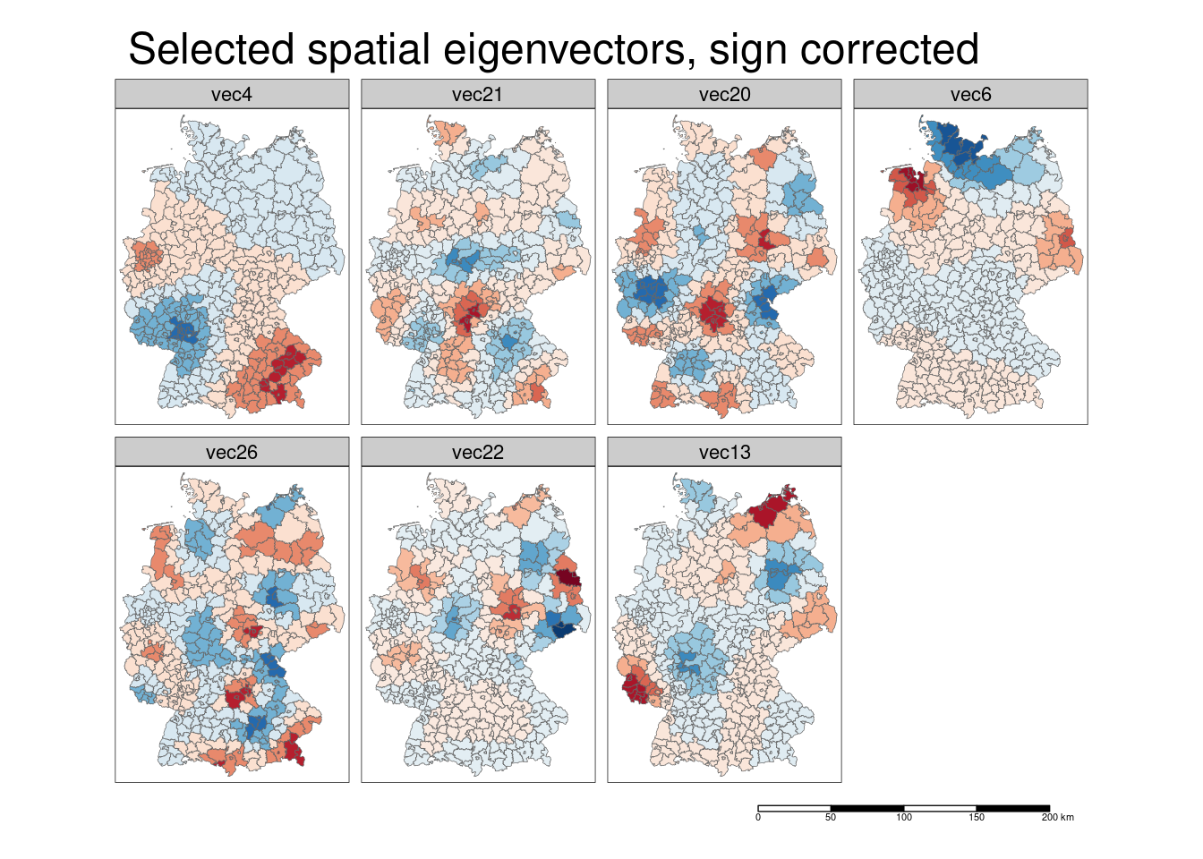
tm_shape(covidKreiseSvem) +
  tm_polygons(col= sevNamesEffect, palette = "-RdBu", lwd=.5,
             n = 7, midpoint=1,  legend.show = TRUE, title="Effect at\nresponse scale") +
  tm_layout(main.title = "Selected spatial eigenvectors, effect", legend.outside = TRUE,
            attr.outside = TRUE, panel.show = TRUE,
            panel.labels = colnames(sevQp), title.size = .7) +
  tm_scale_bar()
## ## ── tmap v3 code detected ───────────────────────────────────────────────────────## [v3->v4] `tm_tm_polygons()`: migrate the argument(s) related to the scale of
## the visual variable `fill` namely 'n', 'midpoint', 'palette' (rename to
## 'values') to fill.scale = tm_scale(<HERE>).
## ℹ For small multiples, specify a 'tm_scale_' for each multiple, and put them in
## a list: 'fill.scale = list(<scale1>, <scale2>, ...)'
## [v3->v4] `tm_polygons()`: migrate the argument(s) related to the legend of the
## visual variable `fill` namely 'title' to 'fill.legend = tm_legend(<HERE>)'
## [v3->v4] `tm_layout()`: use `tm_title()` instead of `tm_layout(title = )`
## [v3->v4] `tm_layout()`: use `tm_title()` instead of `tm_layout(main.title = )`
## ! `tm_scale_bar()` is deprecated. Please use `tm_scalebar()` instead.
## Multiple palettes called "rd_bu" found: "brewer.rd_bu", "matplotlib.rd_bu". The first one, "brewer.rd_bu", is returned.
##
## [cols4all] color palettes: use palettes from the R package cols4all. Run
## `cols4all::c4a_gui()` to explore them. The old palette name "-RdBu" is named
## "rd_bu" (in long format "brewer.rd_bu")
## Multiple palettes called "rd_bu" found: "brewer.rd_bu", "matplotlib.rd_bu". The first one, "brewer.rd_bu", is returned.
##
## Multiple palettes called "rd_bu" found: "brewer.rd_bu", "matplotlib.rd_bu". The first one, "brewer.rd_bu", is returned.
##
## Multiple palettes called "rd_bu" found: "brewer.rd_bu", "matplotlib.rd_bu". The first one, "brewer.rd_bu", is returned.
##
## Multiple palettes called "rd_bu" found: "brewer.rd_bu", "matplotlib.rd_bu". The first one, "brewer.rd_bu", is returned.
##
## Multiple palettes called "rd_bu" found: "brewer.rd_bu", "matplotlib.rd_bu". The first one, "brewer.rd_bu", is returned.
##
## Multiple palettes called "rd_bu" found: "brewer.rd_bu", "matplotlib.rd_bu". The first one, "brewer.rd_bu", is returned.
##
## [plot mode] legend/component: Some components or legends are too "high" and are
## therefore rescaled.
## ℹ Set the tmap option `component.autoscale = FALSE` to disable rescaling.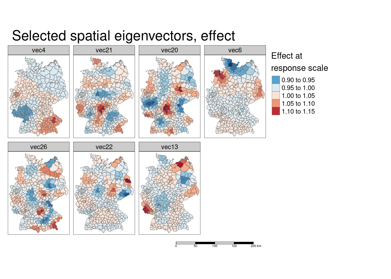
We can also calculate the combined effect of all spatial eigenvectors by taking the product of the effects (at response scale) of the individual eigenvectors.[Remember, the effect is multiplicative at response scale for the log-link function being used.]
covidKreiseSvem$sevEffectResponseProd <- apply(st_drop_geometry(covidKreiseSvem[, sevNamesEffect]), MARGIN= 1, FUN=prod)tm_shape(covidKreiseSvem) +
tm_polygons(col= "sevEffectResponseProd", palette = "-RdBu", lwd=.5,
n = 7, midpoint=1, legend.show = TRUE, title="Combined effect at\nresponse scale") +
tm_layout(main.title = "Selected spatial eigenvectors", legend.outside = TRUE,
attr.outside = TRUE, panel.show = TRUE,
title.size = .7) +
tm_scale_bar()## ## ── tmap v3 code detected ───────────────────────────────────────────────────────## [v3->v4] `tm_tm_polygons()`: migrate the argument(s) related to the scale of
## the visual variable `fill` namely 'n', 'midpoint', 'palette' (rename to
## 'values') to fill.scale = tm_scale(<HERE>).
## ℹ For small multiples, specify a 'tm_scale_' for each multiple, and put them in
## a list: 'fill.scale = list(<scale1>, <scale2>, ...)'
## [v3->v4] `tm_polygons()`: migrate the argument(s) related to the legend of the
## visual variable `fill` namely 'title' to 'fill.legend = tm_legend(<HERE>)'
## [v3->v4] `tm_layout()`: use `tm_title()` instead of `tm_layout(title = )`
## [v3->v4] `tm_layout()`: use `tm_title()` instead of `tm_layout(main.title = )`
## ! `tm_scale_bar()` is deprecated. Please use `tm_scalebar()` instead.
## Multiple palettes called "rd_bu" found: "brewer.rd_bu", "matplotlib.rd_bu". The first one, "brewer.rd_bu", is returned.
##
## [cols4all] color palettes: use palettes from the R package cols4all. Run
## `cols4all::c4a_gui()` to explore them. The old palette name "-RdBu" is named
## "rd_bu" (in long format "brewer.rd_bu")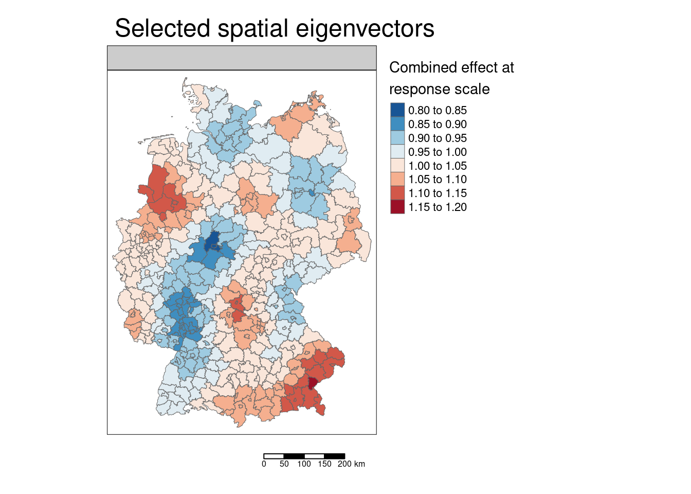
12.3.4 Rechecking spatial autocorrelation
##
##  Global Moran I for regression residuals
##
## data:
## model: glm(formula = sumCasesTotal ~ Stimmenanteile.AfD +
## Auslaenderanteil + Hochqualifizierte + Langzeitarbeitslosenquote +
## Einpendler + fitted(meQp), family = quasipoisson, data = covidKreise,
## offset = log(EWZ))
## weights: unionedListw_d
##
## Moran I statistic standard deviate = 5.7965, p-value = 3.386e-09
## alternative hypothesis: greater
## sample estimates:
## Observed Moran I      Expectation         Variance
##     1.226423e-01    -3.889935e-07     4.476652e-04
modelGlmQp <- glm(sumCasesTotal ~ Stimmenanteile.AfD + Auslaenderanteil +
Hochqualifizierte + Langzeitarbeitslosenquote +
Einpendler + Studierende + offset(log(EWZ)),
data= covidKreise, family = quasipoisson)
moranGlmQp <- lm.morantest(modelGlmQp, listw = unionedListw_d)We see that were is still some left over spatial autocorrelation not absorbed by the spatial eigenvectors. However, the amount of spatial autocorrelation has been reduced by a strong degree, from 0.37 for the normal GLM to 0.12 for the GLM with spatial eigenvector mapping.
12.3.5 Comparison with non spatial GLM
Another question is if the regression coefficients changed:
##               (Intercept)        Stimmenanteile.AfD          Auslaenderanteil
##             -1.2290435997              0.0181073660              0.0082460642
##         Hochqualifizierte Langzeitarbeitslosenquote                Einpendler
##             -0.0051200895             -0.0576477446             -0.0016708665
##               Studierende
## 0.0002804845## (Intercept) Stimmenanteile.AfD Auslaenderanteil
## -1.291694049 0.018531686 0.009665563
## Hochqualifizierte Langzeitarbeitslosenquote Einpendler
## -0.002084850 -0.057739626 -0.001484312
## fitted(meQp)vec4 fitted(meQp)vec21 fitted(meQp)vec20
## -0.858288305 -0.548960968 -0.546537691
## fitted(meQp)vec6 fitted(meQp)vec26 fitted(meQp)vec22
## 0.224236035 -0.287910191 -0.306351870
## fitted(meQp)vec13
## 0.379548226Most coefficients have hardly changed there size. The only exception being the share of highly qualified workers which coefficient is now two time smaller (and only marginally significant as we have seen above.) Ahd of coure the share of students has been dropped by the incorporation of spatial autocorrelation in the model.
We could have a look at the residuals of the spatial eigenvector mapping enhanced GLM to get a better feeling on the left over information in the model:
## Warning: st_point_on_surface assumes attributes are constant over geometrieskreisePoS$residSevmQp <- residuals(modelSevmQp)
kreisePoS$residSevmQpAbs <- abs(kreisePoS$residSevmQp)
tm_shape(covidKreise) +
tm_polygons(col="grey") +
tm_shape(kreisePoS) +
tm_bubbles(size = "residSevmQpAbs", col= "residSevmQp", palette = "-RdBu",
alpha=.9, perceptual=TRUE, scale=.8, border.alpha=.3,
title.size = "Abs residual", title.col="Residuals", n=7,
midpoint = 0) +
tm_layout(main.title = "Pearson residuals, SEVM QP", bg="darkgrey",
legend.outside = TRUE, attr.outside = TRUE) +
tm_scale_bar()## ## ── tmap v3 code detected ───────────────────────────────────────────────────────## [v3->v4] `tm_tm_bubbles()`: migrate the argument(s) related to the scale of the
## visual variable `fill` namely 'n', 'midpoint', 'palette' (rename to 'values')
## to fill.scale = tm_scale(<HERE>).
## ℹ For small multiples, specify a 'tm_scale_' for each multiple, and put them in
## a list: 'fill.scale = list(<scale1>, <scale2>, ...)'
## [v3->v4] `tm_bubbles()`: use `fill_alpha` instead of `alpha`.
## [v3->v4] `tm_bubbles()`: use `col_alpha` instead of `border.alpha`.
## [v3->v4] `tm_bubbles()`: migrate the argument(s) related to the legend of the
## visual variable `fill` namely 'title.col' (rename to 'title') to 'fill.legend =
## tm_legend(<HERE>)'
## [v3->v4] `tm_tm_bubbles()`: migrate the argument(s) related to the scale of the
## visual variable `size` namely 'scale' (rename to 'values.scale') to size.scale
## = tm_scale_continuous(<HERE>).
## ℹ For small multiples, specify a 'tm_scale_' for each multiple, and put them in
## a list: 'size.scale = list(<scale1>, <scale2>, ...)'
## [v3->v4] `tm_layout()`: use `tm_title()` instead of `tm_layout(main.title = )`
## ! `tm_scale_bar()` is deprecated. Please use `tm_scalebar()` instead.
## Multiple palettes called "rd_bu" found: "brewer.rd_bu", "matplotlib.rd_bu". The first one, "brewer.rd_bu", is returned.
##
## [cols4all] color palettes: use palettes from the R package cols4all. Run
## `cols4all::c4a_gui()` to explore them. The old palette name "-RdBu" is named
## "rd_bu" (in long format "brewer.rd_bu")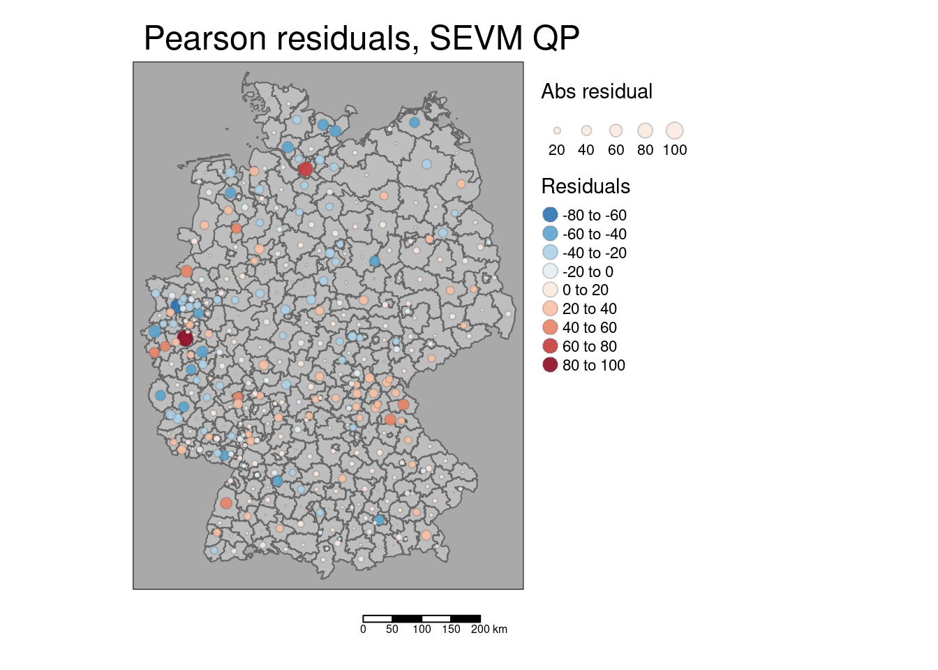
The map shows that the model under- and overpredicts for different regions e.g. in the region between Bavaria, Thuringia and Saxony-Anhalt. Larger residuals however seem not to cluster. The model is overestimating the incidence strongest for the following districts:
st_drop_geometry(kreisePoS) %>%
  slice_min(order_by = residSevmQp, n = 10) %>%
  dplyr::select(GEN, residSevmQp)
## GEN residSevmQp
## 1 Duisburg -69.45758
## 2 Heinsberg -58.08948
## 3 Rhein-Sieg-Kreis -52.37796
## 4 Ostholstein -51.97746
## 5 Steinburg -49.52292
## 6 Plön -47.54910
## 7 Ammerland -43.98155
## 8 Stuttgart -43.41315
## 9 Magdeburg -43.41234
## 10 Bernkastel-Wittlich -42.86121The model is underestimating the incidence strongest for the following districts:
st_drop_geometry(kreisePoS) %>%
  slice_max(order_by = residSevmQp, n = 10) %>%
  dplyr::select(GEN, residSevmQp)
## GEN residSevmQp
## 1 Köln 91.95400
## 2 Hamburg 76.93816
## 3 Borken 55.21081
## 4 Ortenaukreis 52.13172
## 5 Neustadt a.d. Waldnaab 50.42804
## 6 Tirschenreuth 48.78595
## 7 Städteregion Aachen 43.64983
## 8 Vechta 41.86190
## 9 Düren 40.41883
## 10 Wiesbaden 40.0853412.4 Spatially varying regression coefficients
If one includes interactions between the spatial eigenvectors and the predictors in the model it is possible to test for spatially varying regression coefficients. Therefore, we use the sf object with the selected spatial eigenvectors selected covidKreiseSvem.
This of course requires testing a lot of possibilities. We will start checking for spatial varying regression coefficients for the share of foreigners.
modelSevmQpInt <- glm(sumCasesTotal ~ Stimmenanteile.AfD +
    Hochqualifizierte + Langzeitarbeitslosenquote + Einpendler  +
      Auslaenderanteil*(vec4 + vec6 + vec13  + vec20 +  vec21  + vec22 + vec26 ),
                   family = quasipoisson, offset = log(EWZ),
                   data = covidKreiseSvem)
drop1(modelSevmQpInt, test="F")
## Single term deletions
##
## Model:
## sumCasesTotal ~ Stimmenanteile.AfD + Hochqualifizierte + Langzeitarbeitslosenquote +
## Einpendler + Auslaenderanteil * (vec4 + vec6 + vec13 + vec20 +
## vec21 + vec22 + vec26)
## Df Deviance F value Pr(>F)
## <none> 165619
## Stimmenanteile.AfD 1 317756 349.0662 < 2.2e-16 ***
## Hochqualifizierte 1 166440 1.8836 0.1707325
## Langzeitarbeitslosenquote 1 293449 293.2952 < 2.2e-16 ***
## Einpendler 1 172261 15.2384 0.0001121 ***
## Auslaenderanteil:vec4 1 171428 13.3272 0.0002982 ***
## Auslaenderanteil:vec6 1 166900 2.9390 0.0872821 .
## Auslaenderanteil:vec13 1 167618 4.5873 0.0328445 *
## Auslaenderanteil:vec20 1 165947 0.7515 0.3865551
## Auslaenderanteil:vec21 1 166883 2.8998 0.0894093 .
## Auslaenderanteil:vec22 1 165765 0.3343 0.5634708
## Auslaenderanteil:vec26 1 165818 0.4572 0.4993687
## ---
## Signif. codes: 0 '***' 0.001 '**' 0.01 '*' 0.05 '.' 0.1 ' ' 1modelSevmQpInt <- update(modelSevmQpInt, ~. -Auslaenderanteil:vec22)
drop1(modelSevmQpInt, test="F")## Single term deletions
##
## Model:
## sumCasesTotal ~ Stimmenanteile.AfD + Hochqualifizierte + Langzeitarbeitslosenquote +
## Einpendler + Auslaenderanteil + vec4 + vec6 + vec13 + vec20 +
## vec21 + vec22 + vec26 + Auslaenderanteil:vec4 + Auslaenderanteil:vec6 +
## Auslaenderanteil:vec13 + Auslaenderanteil:vec20 + Auslaenderanteil:vec21 +
## Auslaenderanteil:vec26
## Df Deviance F value Pr(>F)
## <none> 165765
## Stimmenanteile.AfD 1 321759 358.5442 < 2.2e-16 ***
## Hochqualifizierte 1 166528 1.7550 0.1860474
## Langzeitarbeitslosenquote 1 294764 296.4962 < 2.2e-16 ***
## Einpendler 1 172346 15.1261 0.0001186 ***
## vec22 1 171386 12.9210 0.0003676 ***
## Auslaenderanteil:vec4 1 171906 14.1152 0.0001988 ***
## Auslaenderanteil:vec6 1 167218 3.3410 0.0683539 .
## Auslaenderanteil:vec13 1 167819 4.7216 0.0304019 *
## Auslaenderanteil:vec20 1 166092 0.7521 0.3863477
## Auslaenderanteil:vec21 1 167091 3.0487 0.0816102 .
## Auslaenderanteil:vec26 1 165904 0.3201 0.5718998
## ---
## Signif. codes: 0 '***' 0.001 '**' 0.01 '*' 0.05 '.' 0.1 ' ' 1modelSevmQpInt <- update(modelSevmQpInt, ~. -Auslaenderanteil:vec26)
drop1(modelSevmQpInt, test="F")## Single term deletions
##
## Model:
## sumCasesTotal ~ Stimmenanteile.AfD + Hochqualifizierte + Langzeitarbeitslosenquote +
## Einpendler + Auslaenderanteil + vec4 + vec6 + vec13 + vec20 +
## vec21 + vec22 + vec26 + Auslaenderanteil:vec4 + Auslaenderanteil:vec6 +
## Auslaenderanteil:vec13 + Auslaenderanteil:vec20 + Auslaenderanteil:vec21
## Df Deviance F value Pr(>F)
## <none> 165904
## Stimmenanteile.AfD 1 321953 359.3093 < 2.2e-16 ***
## Hochqualifizierte 1 166756 1.9622 0.1620885
## Langzeitarbeitslosenquote 1 294960 297.1571 < 2.2e-16 ***
## Einpendler 1 173037 16.4241 6.137e-05 ***
## vec22 1 171825 13.6339 0.0002545 ***
## vec26 1 167801 4.3679 0.0372837 *
## Auslaenderanteil:vec4 1 172630 15.4859 9.875e-05 ***
## Auslaenderanteil:vec6 1 167429 3.5123 0.0616761 .
## Auslaenderanteil:vec13 1 168113 5.0865 0.0246785 *
## Auslaenderanteil:vec20 1 166264 0.8296 0.3629602
## Auslaenderanteil:vec21 1 167462 3.5875 0.0589712 .
## ---
## Signif. codes: 0 '***' 0.001 '**' 0.01 '*' 0.05 '.' 0.1 ' ' 1modelSevmQpInt <- update(modelSevmQpInt, ~. -Auslaenderanteil:vec20)
drop1(modelSevmQpInt, test="F")## Single term deletions
##
## Model:
## sumCasesTotal ~ Stimmenanteile.AfD + Hochqualifizierte + Langzeitarbeitslosenquote +
## Einpendler + Auslaenderanteil + vec4 + vec6 + vec13 + vec20 +
## vec21 + vec22 + vec26 + Auslaenderanteil:vec4 + Auslaenderanteil:vec6 +
## Auslaenderanteil:vec13 + Auslaenderanteil:vec21
## Df Deviance F value Pr(>F)
## <none> 166264
## Stimmenanteile.AfD 1 323584 362.3963 < 2.2e-16 ***
## Hochqualifizierte 1 166889 1.4380 0.2311997
## Langzeitarbeitslosenquote 1 301992 312.6582 < 2.2e-16 ***
## Einpendler 1 174035 17.9000 2.916e-05 ***
## vec20 1 177846 26.6802 3.869e-07 ***
## vec22 1 172481 14.3212 0.0001788 ***
## vec26 1 168045 4.1010 0.0435502 *
## Auslaenderanteil:vec4 1 173246 16.0827 7.291e-05 ***
## Auslaenderanteil:vec6 1 167725 3.3640 0.0674136 .
## Auslaenderanteil:vec13 1 168384 4.8829 0.0277155 *
## Auslaenderanteil:vec21 1 167486 2.8138 0.0942732 .
## ---
## Signif. codes: 0 '***' 0.001 '**' 0.01 '*' 0.05 '.' 0.1 ' ' 1modelSevmQpInt <- update(modelSevmQpInt, ~. -Auslaenderanteil:vec21)
drop1(modelSevmQpInt, test="F")## Single term deletions
##
## Model:
## sumCasesTotal ~ Stimmenanteile.AfD + Hochqualifizierte + Langzeitarbeitslosenquote +
## Einpendler + Auslaenderanteil + vec4 + vec6 + vec13 + vec20 +
## vec21 + vec22 + vec26 + Auslaenderanteil:vec4 + Auslaenderanteil:vec6 +
## Auslaenderanteil:vec13
## Df Deviance F value Pr(>F)
## <none> 167486
## Stimmenanteile.AfD 1 326010 363.4526 < 2.2e-16 ***
## Hochqualifizierte 1 168170 1.5692 0.211087
## Langzeitarbeitslosenquote 1 304468 314.0646 < 2.2e-16 ***
## Einpendler 1 175583 18.5657 2.088e-05 ***
## vec20 1 182018 33.3194 1.614e-08 ***
## vec21 1 184740 39.5589 8.673e-10 ***
## vec22 1 172922 12.4649 0.000465 ***
## vec26 1 169638 4.9342 0.026913 *
## Auslaenderanteil:vec4 1 174461 15.9933 7.626e-05 ***
## Auslaenderanteil:vec6 1 169501 4.6215 0.032197 *
## Auslaenderanteil:vec13 1 169487 4.5882 0.032822 *
## ---
## Signif. codes: 0 '***' 0.001 '**' 0.01 '*' 0.05 '.' 0.1 ' ' 1We should now drop the share of highly qualified workers as well which was only marginally significant beforehand.
## Single term deletions
##
## Model:
## sumCasesTotal ~ Stimmenanteile.AfD + Langzeitarbeitslosenquote +
##     Einpendler + Auslaenderanteil + vec4 + vec6 + vec13 + vec20 +
##     vec21 + vec22 + vec26 + Auslaenderanteil:vec4 + Auslaenderanteil:vec6 +
##     Auslaenderanteil:vec13
##                           Df Deviance  F value    Pr(>F)
## <none>                         168170
## Stimmenanteile.AfD         1   327210 364.0985 < 2.2e-16 ***
## Langzeitarbeitslosenquote  1   304815 312.8267 < 2.2e-16 ***
## Einpendler                 1   175600  17.0095 4.560e-05 ***
## vec20                      1   183948  36.1216 4.303e-09 ***
## vec21                      1   185339  39.3043 9.738e-10 ***
## vec22                      1   173932  13.1913 0.0003193 ***
## vec26                      1   170292   4.8578 0.0281128 *
## Auslaenderanteil:vec4      1   176526  19.1302 1.574e-05 ***
## Auslaenderanteil:vec6      1   170073   4.3563 0.0375284 *
## Auslaenderanteil:vec13     1   170458   5.2381 0.0226381 *
## ---
## Signif. codes:  0 '***' 0.001 '**' 0.01 '*' 0.05 '.' 0.1 ' ' 1
I would tend to also drop the interaction with the spatial eigenvector 6 as it is not highly significant to avoid spurious effects in the model.
## Single term deletions
##
## Model:
## sumCasesTotal ~ Stimmenanteile.AfD + Langzeitarbeitslosenquote +
##     Einpendler + Auslaenderanteil + vec4 + vec6 + vec13 + vec20 +
##     vec21 + vec22 + vec26 + Auslaenderanteil:vec4 + Auslaenderanteil:vec13
##                           Df Deviance  F value    Pr(>F)
## <none>                         170073
## Stimmenanteile.AfD         1   333532 370.9891 < 2.2e-16 ***
## Langzeitarbeitslosenquote  1   305150 306.5717 < 2.2e-16 ***
## Einpendler                 1   177493  16.8414 4.961e-05 ***
## vec6                       1   172503   5.5146 0.0193622 *
## vec20                      1   186806  37.9762 1.803e-09 ***
## vec21                      1   185973  36.0868 4.365e-09 ***
## vec22                      1   175301  11.8663 0.0006343 ***
## vec26                      1   172534   5.5848 0.0186118 *
## Auslaenderanteil:vec4      1   179609  21.6418 4.522e-06 ***
## Auslaenderanteil:vec13     1   173087   6.8398 0.0092644 **
## ---
## Signif. codes: 0 '***' 0.001 '**' 0.01 '*' 0.05 '.' 0.1 ' ' 1##
## Call:
## glm(formula = sumCasesTotal ~ Stimmenanteile.AfD + Langzeitarbeitslosenquote +
## Einpendler + Auslaenderanteil + vec4 + vec6 + vec13 + vec20 +
## vec21 + vec22 + vec26 + Auslaenderanteil:vec4 + Auslaenderanteil:vec13,
## family = quasipoisson, data = covidKreiseSvem, offset = log(EWZ))
##
## Coefficients:
## Estimate Std. Error t value Pr(>|t|)
## (Intercept) -1.3006498 0.0361063 -36.023 < 2e-16 ***
## Stimmenanteile.AfD 0.0186278 0.0009599 19.406 < 2e-16 ***
## Langzeitarbeitslosenquote -0.0575468 0.0033196 -17.336 < 2e-16 ***
## Einpendler -0.0016540 0.0004023 -4.111 4.81e-05 ***
## Auslaenderanteil 0.0089536 0.0009707 9.223 < 2e-16 ***
## vec4 -1.8659753 0.2380709 -7.838 4.50e-14 ***
## vec6 0.2210162 0.0941106 2.348 0.019354 *
## vec13 0.0454272 0.1820724 0.250 0.803106
## vec20 -0.5623243 0.0912149 -6.165 1.78e-09 ***
## vec21 -0.5845771 0.0971993 -6.014 4.20e-09 ***
## vec22 -0.2921727 0.0847857 -3.446 0.000631 ***
## vec26 -0.2235599 0.0945233 -2.365 0.018518 *
## Auslaenderanteil:vec4 0.0737290 0.0158685 4.646 4.64e-06 ***
## Auslaenderanteil:vec13 0.0403695 0.0154582 2.612 0.009366 **
## ---
## Signif. codes: 0 '***' 0.001 '**' 0.01 '*' 0.05 '.' 0.1 ' ' 1
##
## (Dispersion parameter for quasipoisson family taken to be 440.3991)
##
## Null deviance: 555100 on 399 degrees of freedom
## Residual deviance: 170073 on 386 degrees of freedom
## AIC: NA
##
## Number of Fisher Scoring iterations: 4Now the main effect of spatial eigenvector 6 is no longer significantly different from zero, only the interaction with the share of foreigners. It might be worth dropping the interaction - or to test for other interaction of this eigenvector with predictors.
The explained deviance increased a bit by adding the interaction, but not dramatically.
## [1] 0.6936173## [1] 0.6794871Let’s map the resulting regression coefficient for the share of foreigners. This involves some manual calculations
First we map the results of the interaction between foreigners and each of the three eigenvectors.
mForeignerVec4 <- covidKreiseSvem %>%
  mutate(vec4Foreign =  vec4 * Auslaenderanteil) %>%
  tm_shape() + tm_polygons(col=c("vec4Foreign"),
                           legend.hist = TRUE, palette="-RdBu",
                           style = "fisher", n = 6, midpoint = 0,
                         legend.reverse = TRUE,
                         title = "Share foreigners moderated by eigenvector 4") +
  tm_layout(legend.outside = TRUE, bg.color = "darkgrey", outer.bg.color = "lightgrey",
            legend.outside.size = 0.5, attr.outside = TRUE,  legend.outside.position = "left",
            main.title = "Share foreigners by sev 4") +
  tm_scale_bar()
## ## ── tmap v3 code detected ───────────────────────────────────────────────────────## [v3->v4] `tm_polygons()`: instead of `style = "fisher"`, use fill.scale =
## `tm_scale_intervals()`.
## ℹ Migrate the argument(s) 'style', 'n', 'midpoint', 'palette' (rename to
## 'values') to 'tm_scale_intervals(<HERE>)'
## For small multiples, specify a 'tm_scale_' for each multiple, and put them in a
## list: 'fill'.scale = list(<scale1>, <scale2>, ...)'
## [v3->v4] `tm_polygons()`: migrate the argument(s) related to the legend of the
## visual variable `fill` namely 'title', 'legend.reverse' (rename to 'reverse')
## to 'fill.legend = tm_legend(<HERE>)'
## [v3->v4] `tm_polygons()`: use `fill.chart = tm_chart_histogram()` instead of
## `legend.hist = TRUE`.
## [v3->v4] `tm_layout()`: use `tm_title()` instead of `tm_layout(main.title = )`
## ! `tm_scale_bar()` is deprecated. Please use `tm_scalebar()` instead.mForeignerVec13 <- covidKreiseSvem %>%
mutate(vec13Foreign = vec13 * Auslaenderanteil) %>%
tm_shape() + tm_polygons(col=c("vec13Foreign"),
legend.hist = TRUE, palette="-RdBu",
style = "fisher", n = 6, midpoint = 0,
legend.reverse = TRUE,
title = "Share foreigners moderated by eigenvector 13") +
tm_layout(legend.outside = TRUE, bg.color = "darkgrey", outer.bg.color = "lightgrey",
legend.outside.size = 0.5, attr.outside = TRUE, legend.outside.position = "left",
main.title = "Share foreigners by sev 13") +
tm_scale_bar()## [v3->v4] `tm_polygons()`: migrate the argument(s) related to the legend of the
## visual variable `fill` namely 'title', 'legend.reverse' (rename to 'reverse')
## to 'fill.legend = tm_legend(<HERE>)'
## [v3->v4] `tm_layout()`: use `tm_title()` instead of `tm_layout(main.title = )`
## ! `tm_scale_bar()` is deprecated. Please use `tm_scalebar()` instead.mForeigner <- covidKreiseSvem %>%
tm_shape() + tm_polygons(col=c("Auslaenderanteil"),
legend.hist = TRUE,
style = "fisher", n = 6,
legend.reverse = TRUE,
title = "Share of foreigners") +
tm_layout(legend.outside = TRUE, bg.color = "darkgrey", outer.bg.color = "lightgrey",
legend.outside.size = 0.5, attr.outside = TRUE, legend.outside.position = "left",
main.title = "Share of foreigners") +
tm_scale_bar()## [v3->v4] `tm_polygons()`: migrate the argument(s) related to the legend of the
## visual variable `fill` namely 'title', 'legend.reverse' (rename to 'reverse')
## to 'fill.legend = tm_legend(<HERE>)'
## [v3->v4] `tm_layout()`: use `tm_title()` instead of `tm_layout(main.title = )`
## ! `tm_scale_bar()` is deprecated. Please use `tm_scalebar()` instead.## Multiple palettes called "rd_bu" found: "brewer.rd_bu", "matplotlib.rd_bu". The first one, "brewer.rd_bu", is returned.
## [cols4all] color palettes: use palettes from the R package cols4all. Run
## `cols4all::c4a_gui()` to explore them. The old palette name "-RdBu" is named
## "rd_bu" (in long format "brewer.rd_bu")[plot mode] fit legend/component: Some legend items or map compoments do not
## fit well, and are therefore rescaled.
## ℹ Set the tmap option `component.autoscale = FALSE` to disable rescaling.Multiple palettes called "rd_bu" found: "brewer.rd_bu", "matplotlib.rd_bu". The first one, "brewer.rd_bu", is returned.
## [cols4all] color palettes: use palettes from the R package cols4all. Run
## `cols4all::c4a_gui()` to explore them. The old palette name "-RdBu" is named
## "rd_bu" (in long format "brewer.rd_bu")[plot mode] fit legend/component: Some legend items or map compoments do not
## fit well, and are therefore rescaled.
## ℹ Set the tmap option `component.autoscale = FALSE` to disable rescaling.[plot mode] legend/component: Some components or legends are too "high" and are
## therefore rescaled.
## ℹ Set the tmap option `component.autoscale = FALSE` to disable rescaling.
For the interpretation we need of course to take the sign of the regression coefficients into account. We continue by calculating the resulting regression coefficient for each district.
\[ y = \beta_1 * Auslaenderanteil + \beta_2 * Auslaenderanteil * vec4 + + \beta_3 * Auslaenderanteil * vec13 + ... = \] \[ = Auslaenderanteil * (\beta_1 + \beta_2 * vec4 + \beta_3 * vec13 ) + ...\] where \((\beta_1 + \beta_2 * vec4 + \beta_3 * vec13 )\) represents the resulting regression coefficient per district.
covidKreiseSvem %>%
  mutate(coefForeigner = coef(modelSevmQpInt)["Auslaenderanteil"] +
           vec4*coef(modelSevmQpInt)["Auslaenderanteil:vec4"] +
           vec13*coef(modelSevmQpInt)["Auslaenderanteil:vec13"]) %>%
  tm_shape() + tm_polygons(col = "coefForeigner",
                           title = "Regression coefficient",
                           palette = "-RdBu", midpoint= 0, n=6) +
  tm_layout(legend.outside = TRUE, bg.color = "darkgrey", outer.bg.color = "lightgrey",
            legend.outside.size = 0.5, attr.outside = TRUE,  legend.outside.position = "right",
            main.title = "Spatial varying regression coefficient for share foreigners") +
  tm_scale_bar()
## ## ── tmap v3 code detected ───────────────────────────────────────────────────────## [v3->v4] `tm_tm_polygons()`: migrate the argument(s) related to the scale of
## the visual variable `fill` namely 'n', 'midpoint', 'palette' (rename to
## 'values') to fill.scale = tm_scale(<HERE>).
## ℹ For small multiples, specify a 'tm_scale_' for each multiple, and put them in
## a list: 'fill.scale = list(<scale1>, <scale2>, ...)'
## [v3->v4] `tm_polygons()`: migrate the argument(s) related to the legend of the
## visual variable `fill` namely 'title' to 'fill.legend = tm_legend(<HERE>)'
## [v3->v4] `tm_layout()`: use `tm_title()` instead of `tm_layout(main.title = )`
## ! `tm_scale_bar()` is deprecated. Please use `tm_scalebar()` instead.
## Multiple palettes called "rd_bu" found: "brewer.rd_bu", "matplotlib.rd_bu". The first one, "brewer.rd_bu", is returned.
##
## [cols4all] color palettes: use palettes from the R package cols4all. Run
## `cols4all::c4a_gui()` to explore them. The old palette name "-RdBu" is named
## "rd_bu" (in long format "brewer.rd_bu")
## [plot mode] fit legend/component: Some legend items or map compoments do not
## fit well, and are therefore rescaled.
## ℹ Set the tmap option `component.autoscale = FALSE` to disable rescaling.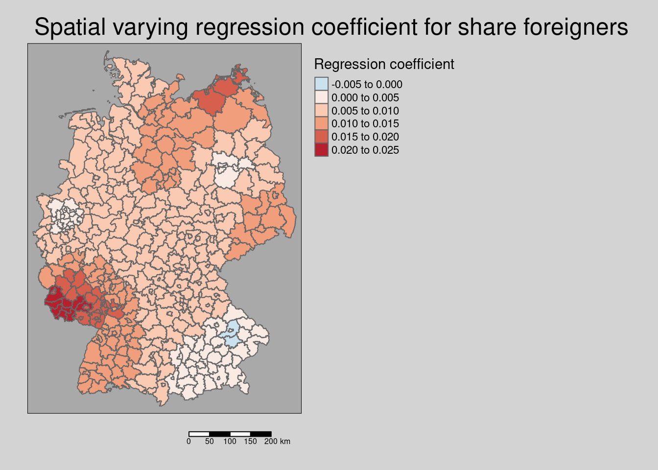
We see that the share of foreigners is with two exceptions in Bavaria always associated with higher incidence rates. The strength of this relationship varies in space. This might reflect the different communities formed by foreigners (different education, integration, language,…) as well as how well the different groups of foreigners are addressed by e.g. the health administration.
The effect on incidence rates is largest in the western parts of Rhineland-Palatina and the Saarland and in parts of Mecklenburg-West Pomerania. The effect was weak in south-east Bavaria, Berlin and the Ruhrgebiet.
covidKreiseSvem %>%
  mutate(coefForeigner = coef(modelSevmQpInt)["Auslaenderanteil"] +
           vec4*coef(modelSevmQpInt)["Auslaenderanteil:vec4"] +
           vec13*coef(modelSevmQpInt)["Auslaenderanteil:vec13"]) %>%
  slice_min( order_by = coefForeigner, n=2) %>%
  dplyr::select(GEN, coefForeigner)
## Simple feature collection with 2 features and 2 fields
## Geometry type: MULTIPOLYGON
## Dimension: XY
## Bounding box: xmin: 729775.8 ymin: 5375702 xmax: 792406.6 ymax: 5447459
## Projected CRS: ETRS89 / UTM zone 32N
## GEN coefForeigner geom
## 1 Dingolfing-Landau -0.0001543393 MULTIPOLYGON (((775571.6 54...
## 2 Straubing-Bogen -0.0001370665 MULTIPOLYGON (((772729.9 54...covidKreiseSvem %>%
mutate(coefForeigner = coef(modelSevmQpInt)["Auslaenderanteil"] +
vec4*coef(modelSevmQpInt)["Auslaenderanteil:vec4"] +
vec13*coef(modelSevmQpInt)["Auslaenderanteil:vec13"]) %>%
slice_max( order_by = coefForeigner, n=15) %>%
dplyr::select(GEN, coefForeigner) ## Simple feature collection with 15 features and 2 fields
## Geometry type: MULTIPOLYGON
## Dimension: XY
## Bounding box: xmin: 308753.6 ymin: 5431733 xmax: 427681.2 ymax: 5532019
## Projected CRS: ETRS89 / UTM zone 32N
## First 10 features:
## GEN coefForeigner geom
## 1 Neunkirchen 0.02185477 MULTIPOLYGON (((354645.1 54...
## 2 Saarpfalz-Kreis 0.02145253 MULTIPOLYGON (((376469 5473...
## 3 St. Wendel 0.02114215 MULTIPOLYGON (((359841 5499...
## 4 Kusel 0.02079128 MULTIPOLYGON (((394474.5 55...
## 5 Zweibrücken 0.02071701 MULTIPOLYGON (((383498 5463...
## 6 Regionalverband Saarbrücken 0.02062511 MULTIPOLYGON (((350868.7 54...
## 7 Trier-Saarburg 0.02054645 MULTIPOLYGON (((335248 5531...
## 8 Kaiserslautern 0.02053635 MULTIPOLYGON (((409049.6 54...
## 9 Saarlouis 0.02050314 MULTIPOLYGON (((348671.9 54...
## 10 Merzig-Wadern 0.02004259 MULTIPOLYGON (((347746.9 54...We could as well check out the multiplicative effect of the regression coefficients at response scale.
covidKreiseSvem %>%
  mutate(coefForeignerResp = exp( coef(modelSevmQpInt)["Auslaenderanteil"] +
           vec4*coef(modelSevmQpInt)["Auslaenderanteil:vec4"] +
           vec13*coef(modelSevmQpInt)["Auslaenderanteil:vec13"])) %>%
  tm_shape() + tm_polygons(col = "coefForeignerResp",
                           title = "Regression coefficient,\nresponse scale",
                           palette = "-RdBu", midpoint= 1, n=6) +
  tm_layout(legend.outside = TRUE, bg.color = "darkgrey", outer.bg.color = "lightgrey",
            legend.outside.size = 0.5, attr.outside = TRUE,  legend.outside.position = "right",
            main.title = "Spatial varying regression coefficient\n for share foreigners",
            title.size = .5) +
  tm_scale_bar()
## ## ── tmap v3 code detected ───────────────────────────────────────────────────────## [v3->v4] `tm_tm_polygons()`: migrate the argument(s) related to the scale of
## the visual variable `fill` namely 'n', 'midpoint', 'palette' (rename to
## 'values') to fill.scale = tm_scale(<HERE>).
## ℹ For small multiples, specify a 'tm_scale_' for each multiple, and put them in
## a list: 'fill.scale = list(<scale1>, <scale2>, ...)'
## [v3->v4] `tm_polygons()`: migrate the argument(s) related to the legend of the
## visual variable `fill` namely 'title' to 'fill.legend = tm_legend(<HERE>)'
## [v3->v4] `tm_layout()`: use `tm_title()` instead of `tm_layout(title = )`
## [v3->v4] `tm_layout()`: use `tm_title()` instead of `tm_layout(main.title = )`
## ! `tm_scale_bar()` is deprecated. Please use `tm_scalebar()` instead.
## Multiple palettes called "rd_bu" found: "brewer.rd_bu", "matplotlib.rd_bu". The first one, "brewer.rd_bu", is returned.
##
## [cols4all] color palettes: use palettes from the R package cols4all. Run
## `cols4all::c4a_gui()` to explore them. The old palette name "-RdBu" is named
## "rd_bu" (in long format "brewer.rd_bu")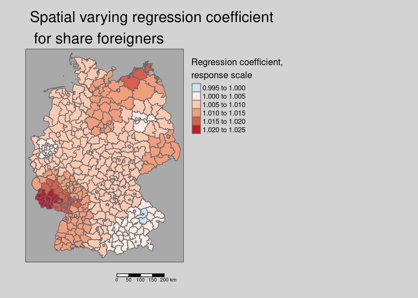
Of course there is much more potential to explore relationships between predictors and spatial eigenvectors and we have not even touched on interactions between “normal” predictors or higher order effects. We could (and should) try other predictor eigenvector combinations as well as interactions between the predictors.