Chapter 10 Non spatial regression analysis
Before we use spatial regression approaches what deal with the challenge of spatial autocorrelation, we need to first start with an ordinary non-spatial regression analysis. For the COVID-19 case study we need to address thereby the following issues:
- the data are count data which calls for a generalized linear model (GLM) with a Poisson distribution as a staring point
- we need to consider the different population at risk by means of an offset
- we need to check for overdispersion and potentially use a quasipoisson or negative binomial GLM
- we need to compare (not necessarily nested) models of different complexity by likelihood measures such as AIC or BIC
- for quasipoisson models with have the additional nuisance that no likelihood is defined and that we have to rely on F-tests which are limited to nested models
This section aims at providing the necessary background and show the use of the methods at the example of the COVID-19 dataset that we used before.
10.1 Cheat sheet
## Loading required package: knitr## Loading required package: sf## Linking to GEOS 3.12.1, GDAL 3.8.4, PROJ 9.4.0; sf_use_s2() is TRUE## Loading required package: spdep## Loading required package: spData## To access larger datasets in this package, install the spDataLarge
## package with: `install.packages('spDataLarge',
## repos='https://nowosad.github.io/drat/', type='source')`## Loading required package: tmap## Loading required package: ggplot2## Loading required package: ggpubr## Loading required package: dplyr##
## Attaching package: 'dplyr'## The following objects are masked from 'package:stats':
##
## filter, lag## The following objects are masked from 'package:base':
##
## intersect, setdiff, setequal, union## Loading required package: corrplot## corrplot 0.95 loaded## Loading required package: MASS##
## Attaching package: 'MASS'## The following object is masked from 'package:dplyr':
##
## select## Loading required package: GGally## Registered S3 method overwritten by 'GGally':
## method from
## +.gg ggplot2## Loading required package: ggeffects##
## Attaching package: 'ggeffects'## The following object is masked from 'package:spData':
##
## coffee_data## Loading required package: sjPlot## #refugeeswelcomeMost important functions used:
glm- fit a generalized linear model, do not forget to specify thefamilyargumentMASS::glm.nb- fitting a negative binomial GLMAIC- returns the AIC of a modeldrop1- drops on term at a time and returns the AIC or a test statistic
10.2 Theory
10.2.1 Generalized linear models
Generalized linear models are an extension of the linear model in the sense that they allow us to deal with data that follows different distributions. The framework of the generalized linear model (GLM) allows us to use similar tools and techniques to the linear case.
To define a GLM we need to consider the following three aspects:
- choosing a distribution for the response variable - that implies a distribution for the error term
- defining the systematic part of the model, i.e. defining the predictors to be used
- choosing a link function between the expected value of the response and the systematic part of the model.
The link function \(\eta\) linearizes the relationship between the response and the predictors:
\[ \eta(x_1, x_2,...x_n) = \beta_0 + \beta_1 x_1 + \beta_2 x_2 + ... \beta_n x_n + \epsilon \]
where \(x_1, x_2,... x_n\) are vectors of covariates and \(\beta_0, \beta_1,..., \beta_n\) are the regression coefficients to the estimated.
Besides \(\eta\), the equation of the GLM is similar to the LM - \(\eta\) is also called the linear predictor.
Not every functional relationship can be linearised - the GLM approach is valid for the functions that belong to the exponential family. The exponential family describes distributions that follow the following structure:
\[ f(y; \Theta, \phi) = e^{\frac{y \Theta - b(\Theta)}{a(\phi)} + c(y,\Theta) } \]
Using high school math to analyse the first- and second-order derivatives of equation we get the following equations for the mean and the variance of or response y:
\[E(y) = b'(\Theta) \]
\[ var(y) = b''(\Theta) a(\phi) \]
In the Gaussian model we have seen so far - the linear model belongs to the exponential family as well - we have \(\Theta = \mu\), \(\phi = \sigma^2\), \(a(\phi) = \phi\), \(b(\Theta) = \Theta /2\) and \(c(y,\phi) = - (y^2/\phi + log(2\pi\phi))/2\) which gives us \(E(y) = \mu\) and \(var(y) = \sigma^2\).
For each of the members of the exponential family we can write down the likelihood function and maximize the likelihood given the data. For the LM this maximization has led to the ordinary least squares estimate. For the other members of the exponential family we get different maximization criteria which can all be shown to be equivalent to iteratively re-weighted least squares (McCullagh and Nelder, 1989). The iteratively re-weighting is necessary since the variance is in most cases no longer constant as in the Gaussian case but varies with the mean.
The link function describes how the mean response \(E(y)= \mu\) is linked to the predictors through the linear predictor \(\eta = g(\mu)\). For each member of the exponential family at least one link function exist, which is called the canonical link which is defined as \(\eta = g(\mu) = \Theta\) but other links exist and are used as well. The most important members of the exponential family together with their canonical link and their variance function are summarized in table.
| Family | Canonical link | Variance function | Type of data |
|---|---|---|---|
| Normal/Gauss | \(\eta = \mu\) | 1 | Continuous |
| Poisson | \(\eta = log \mu\) | \(\mu\) | Counts and density |
| Negative binomial | \(\eta = \mu\) | \(\mu + \frac{\mu^2}{k}\) | Over dispersed count and density |
| Geometric | \(\eta = \mu\) | \(\mu + \mu^2\) | Over dispersed count and density |
| Binomial | \(\eta = log\frac{\mu}{1-\mu}\) | \(\mu(1-\mu)\) | Proportional datav |
| Bernoulli | \(\eta = N log\frac{\mu}{1-\mu}\) | \(N \mu(1-\mu)\) | Presence absence data |
| Gamma | \(\eta = \mu^{-1}\) | \(\frac{\mu^2}{\nu}\) | Continuous |
| Inverse Gaussian | \(\eta = \mu^{-2}\) | \(\frac{\mu^3}{\nu}\) | Lifetime distributions with monotone failure rates |
Other members of the exponential family are the chi-square, the beta, the Dirichlet and the multi-nomial distribution as well as the Weibull distribution - if the shape parameter is known for the latter. Examples for random distributions that do not belong to the exponential family are the Cauchy and uniform families, the Weibull distribution if the shape parameter is not known as well as the distributions of the Laplace family unless the mean is zero.
10.2.2 The deviance of the generalized linear models
In the linear model we are used to quantify the quality of the fit as the sum of the squared residuals, that is
\[ deviance = \sum_i^n{(y_{obs,i}-y_{pred,i})^2} \]
This calculation is only valid if we assume a normally distributed error term. For other distributions we have to calculate the deviance differently.
| Family | Deviance |
|---|---|
| Normal/Gauss: | \(\sum (y-\hat{y})^2\) |
| Poisson: | \(2 \sum (y \cdot log(\frac{y}{\hat{y}}) - (y-\hat{y}))\) |
| Binomial: | \(2 \sum (y \cdot log(\frac{y}{\hat{y}}) + (m-y) log(\frac{m-y}{m-\hat{y}} )\) |
| Gamma: | \(2 \sum ( -log(\frac{y}{\hat{y}}) + \frac{(y-\hat{y}}{\hat{y}})\) |
| Inverse Gaussian: | \(\sum \frac{(y-\hat{y})^2}{\hat{y}^2y}\) |
| Negative binomial (NB2): | \(2 \sum (y \cdot log(\frac{y}{\mu}) - (y + k^{-1}) log(\frac{y+k^{-1}}{\mu + k^{-1}}))\) |
The deviance can be used to calculate pseudo-\(R^2\)s, e.g. the explained deviance defined as:
\[\mbox{explained deviance} = 1 - \frac{\mbox{model deviance}}{\mbox{null model deviance}}\] The null model is (as for the linear model) a model with only the intercept.
10.2.2.1 Plots for the different deviance functions
To give you a better feeling for how the deviance differs for different distribution we plot a few.
10.2.2.1.1 Poisson deviance
For the poisson, the deviance depends not only on the difference between \(y\) and \(\hat{y}\) but also on the value of \(y\) (the meann). We plot the deviance for two different mean vaules and varying estimated \(\hat{y}\) values.
devPois <- function(x, lambda)
{
  return(lambda * log(lambda/x) - (lambda -x))
}
lambda <- 2
p1 <- ggplot() + xlim(0,20) +
  geom_function(fun = devPois, args=list(lambda = lambda)) +
  geom_vline(xintercept = lambda, lty=2, colour =" darkgrey") +
  xlab("estimated y") + ylab("Poisson deviance") + labs(title= paste("Poisson deviance for y =", lambda))

p2 <- ggplot(transform(data.frame(x=c(0:20)), y= dpois(x, lambda)), aes(x,y )) +  geom_bar(stat = "identity")  +
  xlab("y") + ylab("Frequency") + labs(title= paste("Poisson distribution for y =", lambda))
ggarrange(p1,p2)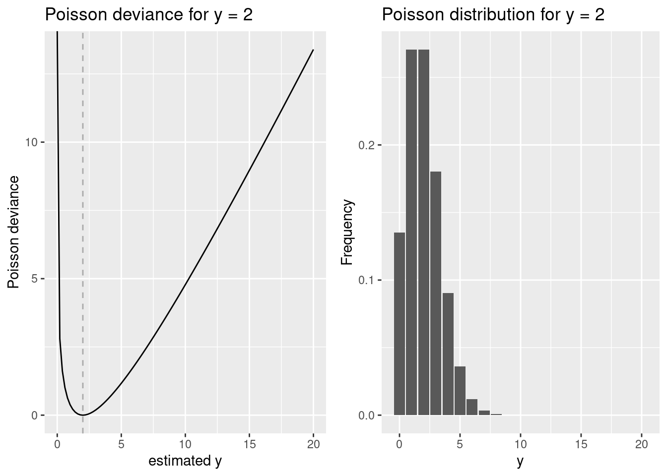
The deviance is zero if \(y\) and \(\hat{y}\) are equal (for 2). The larger the difference between \(y\) and \(\hat{y}\), the larger the deviance - but the relationship is clearly non-linear and non-symmetric.
lambda <- 4
p1 <- ggplot() + xlim(0,20) +
  geom_function(fun = devPois, args=list(lambda = lambda)) +
  geom_vline(xintercept = lambda, lty=2, colour =" darkgrey") +
  xlab("estimated y") + ylab("Poisson deviance") + labs(title= paste("Poisson deviance for y =", lambda))

p2 <- ggplot(transform(data.frame(x=c(0:20)), y= dpois(x, lambda)), aes(x,y )) +  geom_bar(stat = "identity")  +
  xlab("y") + ylab("Frequency") + labs(title= paste("Poisson distribution for y =", lambda))
ggarrange(p1,p2)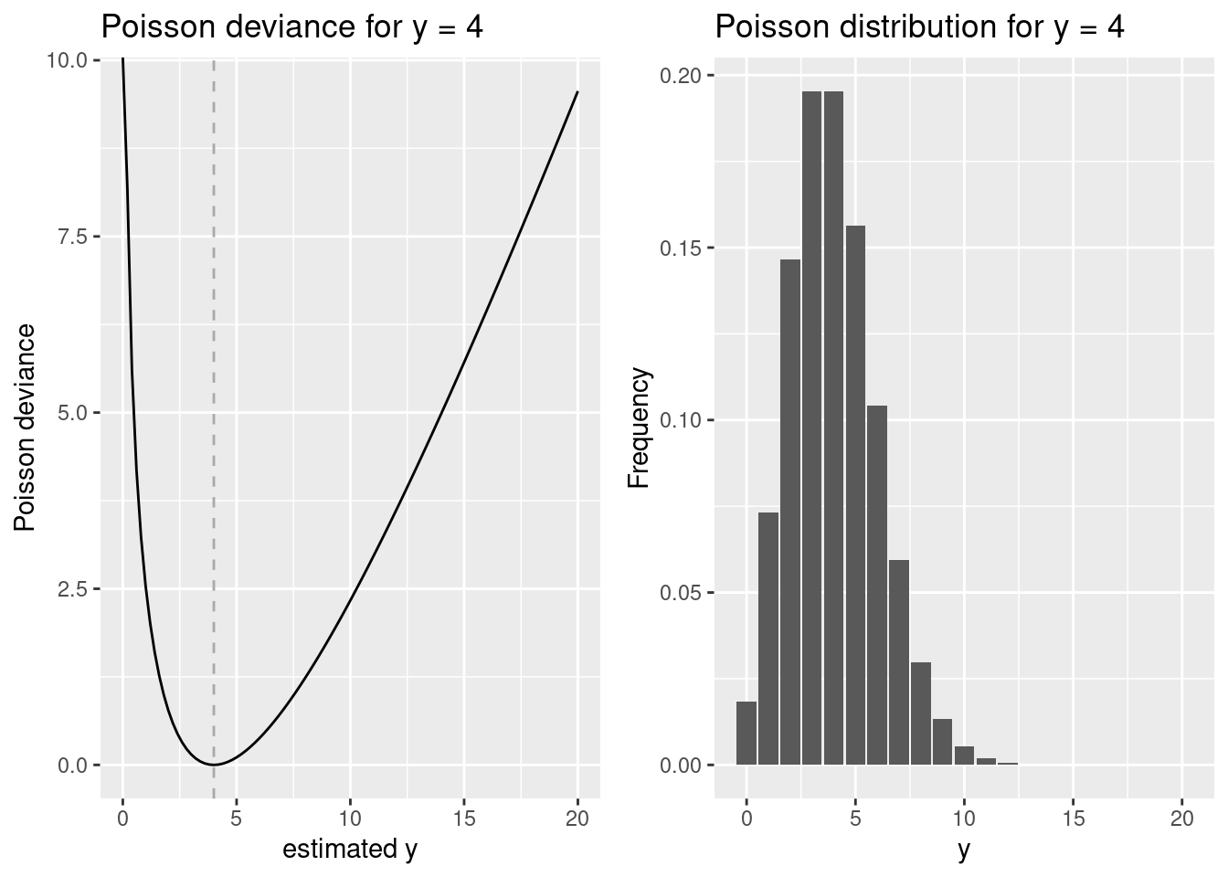
lambda <- 50
p1 <- ggplot() + xlim(0,150) +
  geom_function(fun = devPois, args=list(lambda = lambda)) +
  geom_vline(xintercept = lambda, lty=2, colour =" darkgrey") +
  xlab("estimated y") + ylab("Poisson deviance") + labs(title= paste("Poisson deviance for y =", lambda))

p2 <- ggplot(transform(data.frame(x=c(0:100)), y= dpois(x, lambda)), aes(x,y )) +  geom_bar(stat = "identity")  +
  xlab("y") + ylab("Frequency") + labs(title= paste("Poisson distribution for y =", lambda))
ggarrange(p1,p2)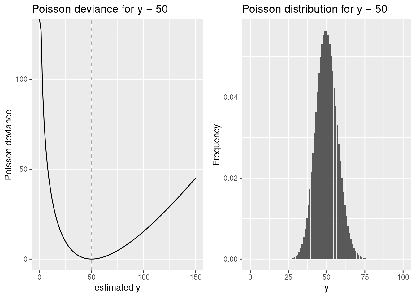
10.2.3 Count regression
10.2.3.1 Poisson GLM
The Poisson regression is commonly used for count data. Our response \(Y_i\) is Poisson distributed with mean \(\mu_i\), the variance is equal to the mean.
The systematic part of the model is given by:\ \[ \eta(x_{i1}, x_{i2}, ...,x_{in}) = \beta_0 + \beta x_{i1} + \beta_2 x_{i2} + ... + \beta_n x_{in}\]
For the link function we usually choose the logarithmic link, i.e. \(log(\mu_i) =\eta(x_{i1}, x_{i2}, ...,x_{in})\).
Together, these three settings give us the following GLM:\
\[ Y_i \quad \widetilde{~} \quad P(\mu_i)\]
\[E[Y_i] = \mu_i \qquad var(Y_i) = \mu_i \] \[ log(\mu_i) =\eta(x_{i1}, x_{i2}, ...,x_{in}) \leftrightarrow \mu_i = e^{\eta(x_{i1}, x_{i2}, ...,x_{in})} = e^{\beta_0 + \beta_1 x_{i1} + \beta_2 x_{i2} + ... \beta_n x_{in}}\]
Coefficients are estimated at the link scale, not the response scale. To make sense out of the coefficients we need to keep in mind that we need to transform the coefficient by taking the anti log (exp) and that the effect is multiplicative.
Let’s look at a simple example. Say we are interested in the number of people (count) who vote for leave in the brexit vote. And let’s assume for a moment that all voting districts would have the same number of voters of 10,000. We tested if the share of unqualified inhabitants [%] has an effect to the outcome (the number of votes). And assume we got the following regression coefficients (assuming the \(\beta_1\) is significantly different from zero):
- \(\beta_0\) (intercept): 8.517193
- \(\beta_1\) (share unqualified inh.): 0.01
What is the effect of the outcome?
You should remember school math with respect of how to work with exponents if the base is the same to make sense out of the following equations. Especially the following:
\[ a^{b+c} = a^b * a ^c \] \[ a^{b-c} = \frac{a^b} {a^c} \]
\[ (a^b)^c = a^{b * c} \]
If we look at a hypothetical district with no unqualified workers the effect is as follows:
\[voteCount = e^{8.517193 + 0 * 0.01} = e ^{8.517193} * e^{0} = e^{8.517193} * 1\]
## [1] 4999.999We expect around half of the population to vote for leave (5000 votes).
Now if we assume a district with 1% of unqualified inhabitants?
\[voteCount = e^{8.517193 + 1 * 0.01} = e ^{8.517193} * e^{0.01} = 4999.999 * 1.01005\]
## [1] 5050.25We expect 5050.25 votes.
Now for a district with 2% share of unqualified workers?
\[voteCount = e^{8.517193 + 2 * 0.01} = e ^{8.517193} * e^{2*0.01} = 4999.999 * (e^{0.01})^2 = 4999.999 * 1.01005^2\]
## [1] 5101.006And for a district with 12% share of unqualified workers?
\[voteCount = e^{8.517193 + 12 * 0.01} = 4999.999 * 1.01005^{12}\]
## [1] 5637.48310.2.3.2 R syntax
Two differences with respect to lm:
- the function is called glm
- we need to specify the family argument (if we don’t do it we still fit a glm with a gaussian distribution)
glm(y~x1+x2, data = yourData, family = poisson)
Commands such as summary, fitted, residuals or predict work as before, but there are a few twists for the interpretation.
10.2.4 Use of an offset in count regression
But what about the real world case that voters between districts differ? We can incorporate this by specifying an offset. An offset is another variable that is included but no regression coefficient is fitted. This is equivalent to fitting the rate but keeping track of the effect of the different population size on variability (as the mean equals the variance).
If we assume, that the number of brexit leave votes is Poisson distributed with a mean $ _i validVotes_i $, where \(\mu_i\) represents the expected number of votes for brexit per valid vote, the expected value is \(E(Y_i) = \mu_i \cdot validVotes_i\) and the variance is $ var(Y_i) = _i validVotes_i $. If we transfer that to the link scale, we get:
\[ E[Y_i] = \mu_i \cdot validVotes_i \] \[ \Rightarrow log(E[Y_i]) = log(\mu_i) + log(validVotes_i) = \beta_0 + \beta_1 x_1 + \beta_2 x_2 + log(validVotes_i) \]
The term \(log(validVotes_i)\) specifies the offset. It does not have an associated regression coefficient, i.e. its relationship with the response is not estimated from the data but specified as a fixed relationship. If we rearrange the equation we see, that we are modelling the rate.
\[ log(E[Y_i]) - log(validVotes_i) = \beta_0 + \beta_1 x_1 + \beta_2 x_2 \] Using the rules for working with logarithms (here: $ log(a) - log(b) = log() $, if the base is the same) this can be rearranged to:
\[ log(\frac{E[Y_i]}{validVotes_i }) = \beta_0 + \beta_1 x_1 + \beta_2 x_2\]
10.2.5 Likelihood based measures for model selection
Often we want to compare models of different complexity. The typical trade-off is as follows: we would like to get a model that is as good as possible (in the sense that it explains the response) but as parsimonious as possible (as less coefficient to be estimated from the data). Having a too complex model raises the risk of overfitting - i.e. the risk of including parameters that have an effect just by chance. This is also called the bias-variance trade-off: we want to predict the response as good as possible but we would like to reduce the variability of a forecast due to overfitting.
\(R^2\) is not a useful measure for model comparison as it does not consider the number of parameters estimated from the data. Several approaches are common: cross-validation, likelihood-ratio tests and likelihood criteria (such as AIC or BIC).
The likelihood ratio test compares the likelihood (\(\mathcal{L}\)) between a larger model \(\Omega\) and a smaller model \(\omega\) which are fitted using the same data:
\[\frac{max_{\Theta \in \Omega} \mathcal{L}(\Theta |y)}{max_{\Theta \in \omega} \mathcal{L}(\Theta |y)} \] where \(max_{\beta,\sigma \in \Omega} \mathcal{L}(\Theta |y)\) is the model with the maximum likelihood for the model with fixed structural component and the model parameters \(\Theta\) (the regression coefficients and other components estimated from the data such as the dispersion parameter (for the quasipoisson or the negative binomial) or the variance (for the normal distribution). The parameters \(\omega\) are a subset of \(\Omega\).
After some manipulation, we get a test that rejects the null hypothesis if:
\[\frac{RSS_\omega - RSS_\Omega}{RSS_\Omega} > \mbox{a constant}\]
Under the assumptions of the linear model, this leads to the following test statistic:
\[F = \frac{RSS_\omega - RSS_\Omega / (p-q)}{RSS_\Omega / (n-p)} \qquad \widetilde{~} \qquad F{p-q,n-p}\]
where p represents the number of parameters in the larger model, q the number of parameters in the smaller model and n the number of data points used to fit the models.
For generalized linear models - with the exception with quasipoisson and quasibinomial models - the likelihood ratio is tested by a \(\chi^2\) distribution:
\[ \mbox{p-value} = P( \chi^2_p \ge -2 \cdot log(r)) \] where \(r\) is the likelihood ratio of the two nested models:
\[r = \frac{\mathcal{L}(\Theta_{model1} |y)}{\mathcal{L}(\Theta_{model2} |y)}\] The degrees of freedom of the \(\chi^2\) distribution \(p = df_{biggerModel} -df_{smallerModel}\), i.e. the number of free parameters in the bigger model minus the free parameters in the smaller model.
If the relative difference in the residual sums of squares is smaller than could be expected by chance we can safely assume that the null hypothesis that both models have the same likelihood is wrong and reject it. In this case we would favor the larger model since it explains more than could be expected by chance alone. Otherwise, we would favor the smaller model since it explains the same by using less parameters.
The likelihood ratio test for two GLMs can be performed in R for example with lmtest::lrtest(model1, model2) or if you want to simplify an existing model by using drop1(model, test="LRT").
The information criteria like the Aikaike Information Criterion (AIC) or the Bayes Information Criterion (BIC) are based the likelihood plus an penalization term which penalizes the number of parameters \(p\):
\[AIC = -2 max \mathcal{L} + 2 \cdot p \]
\[ BIC = -2 max \mathcal{L} + p \cdot log(n) \]
BIC is more conservative than AIC, i.e. tends to favour smaller models. \(n\) is the sample size of the data set.
The AIC or BIC can be used to select models which are fitted on the same data: the smaller the AIC or BIC gets, the better the model. If the \(\Delta AIC\) or \(\Delta BIC\) between two models is smaller than or equal two, the fit of both models can be considered being the same.
There are several things to consider during mode selection:
- You should not eliminate main effects that are part of interactions or appear in higher order terms.
- If the predictors are collinear the model selection will stop too early.
- Stepwise model selection might lead to the wrong model getting selected; a all subset selection is preferable but might not be feasible given the computational burden involved. In addition the problem of multiple testing is amplified.
- The model selection tools do not contain any domain specific knowledge - you might drop another predictor if it makes more sense from domain specific perspective. Generally, it is better to work hypothesis driven if possible. If you use a fishing approach (fit many models, select the best one) you have to think about meaning at the end. For a hypothesis driven approach you need to start thinking from the beginning. Typically the later approach is preferable, especially if you aim for an improved understanding. If your aim is simply good prediction (even if for wrong reasons) fishing might be an option.
- The comparison between two or more models will only be valid if they are fitted to the same dataset; if data are missing for some of the predictors, this assumption might be violated.
- Likelihood ratio tests assume that the models are nested.
AIC and BIC are not standardized, i.e. they can not be used to compare model with different data (response). You can for example not compare two models that you have fitted to different subsets of your data. This is the role of (pseudo-) \(R^2\).
10.2.6 Overdispersion in count GLMs
Overdispersion means that the variance is greater than the mean, i.e. \(var(y_i) = \phi \mu_i\). If \(\phi > 1\) this is called overdispersion, for \(\phi < 1\) we speak of underdispersion. One possibility to check a GLM for overdisperson is to use the \(\chi^2\) approximation of the residual deviance: if there is no overdispersion, then \(D_{\Theta}/\phi\) is \(\chi^2\) distributed with \(n-p\) degress of freedom. Using this we can estimate \(\phi\) as follows:\
\[\hat{\phi} = \frac{D_{\Theta}}{n-p}\]
In R you can get a first estimate for overdispersion (\(\hat{\phi}\)) by
poissonModel$deviance/poissonModel$df.residual
Reasons behind overdispersion can be due to model misspecifications such as missing covariates or interactions, outliers in the response, non-linear effects of covariates misspecified as linear terms or the choice of the wrong link function (Hilbe (2007)). Real overdispersion can exist because the variation in the data is really larger than the mean or due to too many zeros, the clustering of observations or correlations between observations.
If overdispersion occurs in your model, first try to improve the structural part of your model. If this does not help you can move on to quasi-poisson models or to negative binomial models.
10.2.6.1 Quasiposson GLM
Our response \(Y_i\) is distributed with \(E(y_i) = \mu_i\), and the variance is specified by \(var(y_i)=\phi \cdot\mu_i\).
The systematic part of the model is given by:\ \[\eta(x_{i1}, x_{i2}, ...,x_{in}) = \beta_0 + \beta x_{i1} + \beta_2 x_{i2} + ... + \beta_n x_{in}\]
For the link function we choose the logarithmic link, i.e.:
\[ log(\mu_i) =\eta(x_{i1}, x_{i2}, ...,x_{in}) \]
If \(\phi\) is greater than one, we need to correct for overdispersion. This implies refitting the model, estimating the parameter \(\phi\) and doing some other corrections. The introduction of an overdispersion parameter \(\phi\) results in increased standard error: compared to a Poisson model the standard errors are multiplied by the square root of \(\phi\). This implies that marginally significant parameters might become insignificant during the procedure. If the overdispersion is greater than 15 or 20 you should think about using other mehods like negative binomial GLMs or zero-inflated models (Zuur et al. (2009)).
Running a quasi-poisson GLM in R does not involve more than specifying family=quasipoisson:
glm(y~x1+x2+x3, data= yourData, family=quasipoisson)
For quasi-family GLMs we don’t get an AIC as the model can no longer be fitted by a maximum likelihood estimation approach (MLE) but has to use a quasi maximum likelihood approach. But it is possible to use drop1(model, test="F") to compare two nested models. The deviance approach to compare two nested models \(M_1\) (larger model) and \(M_2\) (nested model) uses the following test statistic:
\[ \frac{D_2 - D_1} {\phi(p_1 - p_2)} \qquad \widetilde{~} \qquad F_{p_1-p_2,n-p_1} \]
where \(D_1\) and \(D-2\) are the deviance of the two models, \(\phi\) is the dispersion parameter and \(p_1\) and \(p_2\) are the number of parameters of model 1 and model 2 respectively.
The F-test in drop1 is based on an ANOVA II - this type tests for each main effect after the other main effect.
Coefficient estimates will stay the same GLMs fitter either with family=poisson or family=quasipoisson. What differs are the standard errors as those reflect the additional uncertainty due to overdispersion for the quasipoisson GLM.
The dispersion parameter in summary represents \(\phi\) and therefore gives an estimate of overdispersion. For a Poisson model without overdispersion \(\phi\) should be one.
10.2.6.2 Negative bionmial GLM
For the negative binomial model6 the response is modeled as a Poisson variable with mean \(\lambda\) where the model error is assumed to follow a Gamma distribution. That is why the model is also called the Poisson-Gamma model. Assuming a Gamma distribution for the error allows to model overdispersion in count data. There are two major parametrizations, the NB2 and NB1 form. The NB2 form is commonly used and we refer to this parametrization if using the term negative bionmial model.
The negative binomial GLM can be specified as follows:
Our response \(Y_i\) is negative binomial distributed with mean \(\mu_i\) and parameter \(k\). The variance is equal to \(\mu_i + \mu_i^2/k\).\
The systematic part of the model is given by:
\[\eta(x_{i1}, x_{i2}, ...,x_{in}) = \beta_0 + \beta x_{i1} + \beta_2 x_{i2} + ... + \beta_n x_{in}\]
For the link function we choose the logarithmic link, i.e. \(log(\mu_i) =\eta(x_{i1}, x_{i2}, ...,x_{in})\). The canonical link for the negative binomial would have been the identity function but since we want to ensure that predicted values cannot become negative we have chosen the log-link.\
Together, these three settings give us the following GLM:
\[ Y_i \quad \widetilde{~} \quad NB(\mu_i,k)\\ E(Y_i) = \mu_i \qquad var(Y_i) = \mu_i + \frac{\mu_i^2}{k}\\ log(\mu_i) =\eta(x_{i1}, x_{i2}, ...,x_{in}) \leftrightarrow \mu_i = e^{\eta(x_{i1}, x_{i2}, ...,x_{in})} \]
Compared to the quasipoisson GLM overdispersion is modeled not by a polynomial of first order of the mean but by a quadratic term of the mean. The strength of the quadratic term depends on the parameter \(k\).
To estimate negative binomial GLMs, we use the function glm.nb from the package MASS. We use the logarithmic link (which is the canonical link here) - other available options are the square root link or the identity link.
nbModel <- glm.nb(y ~ x1 + x2, data = yourData, link = "log")
summary(nbModel)
The parameter Theta in the summary output is the parameter \(k\) in equation above. We also get an standard error for Theta but care has to be taken since it does not give a symmetric interval and we are testing on the boundary.
Since we get a likelihood, we can also use the AIC/BIC in the drop1 and add1 commands. If you prefer testing nested models, you can use the \(\chi^2\) test.
10.3 Modelling continuous positive response data
For continuous positive response data such as concentration of pollutants in ground or surface water or in topsoil the gaussian distribution is not well suited as it might produce negative numbers which would make no sense at all. Instead we could use the log-normal distribution, the gamma or the inverse-gaussian distribution. All three are available via the standard glmfunction.
See chapter 11 of (Dunn and Smyth, 2018) for more information.
10.4 Case study count regression
## Reading layer `kreiseWithCovidMeldeWeeklyCleaned' from data source
##   `/home/slautenbach/Documents/lehre/HD/git_areas/spatial_data_science/spatial-data-science/data/covidKreise.gpkg'
##   using driver `GPKG'
## Simple feature collection with 400 features and 145 fields
## Geometry type: MULTIPOLYGON
## Dimension:     XY
## Bounding box:  xmin: 280371.1 ymin: 5235856 xmax: 921292.4 ymax: 6101444
## Projected CRS: ETRS89 / UTM zone 32N## Warning: st_point_on_surface assumes attributes are constant over geometriesdistnb <- dnearneigh(poSurfKreise, d1=1, d2= 70*10^3)
unionedNb <- union.nb(distnb, polynb)
dlist <- nbdists(unionedNb, st_coordinates(poSurfKreise))
dlist <- lapply(dlist, function(x) 1/x)
unionedListw_d <- nb2listw(unionedNb, glist=dlist, style = "W")10.4.1 Mapping of predictors
Let us first create maps og our predictors as this will help us to understand the regression model output better. We also characterize the spatial pattern by means of global Moran’s I. We also list hypothesis of how the predictor might influence the response.
10.4.1.1 Response
First the crude rate of our response:
covidKreise %>%
tm_shape() + tm_polygons(col=c("incidenceTotal"),   legend.hist = TRUE, palette="-plasma",
                         legend.reverse = TRUE, title = "Incidence rate for total period") +
  tm_layout(legend.outside = TRUE, bg.color = "darkgrey", outer.bg.color = "lightgrey",
            legend.outside.size = 0.5, attr.outside = TRUE,
            main.title = "Incidence rate total period") +
  tm_scale_bar()
## ## ── tmap v3 code detected ───────────────────────────────────────────────────────## [v3->v4] `tm_tm_polygons()`: migrate the argument(s) related to the scale of
## the visual variable `fill` namely 'palette' (rename to 'values') to fill.scale
## = tm_scale(<HERE>).
## [v3->v4] `tm_polygons()`: use 'fill' for the fill color of polygons/symbols
## (instead of 'col'), and 'col' for the outlines (instead of 'border.col').
## [v3->v4] `tm_polygons()`: migrate the argument(s) related to the legend of the
## visual variable `fill` namely 'title', 'legend.reverse' (rename to 'reverse')
## to 'fill.legend = tm_legend(<HERE>)'
## [v3->v4] `tm_polygons()`: use `fill.chart = tm_chart_histogram()` instead of
## `legend.hist = TRUE`.
## [v3->v4] `tm_layout()`: use `tm_title()` instead of `tm_layout(main.title = )`
## ! `tm_scale_bar()` is deprecated. Please use `tm_scalebar()` instead.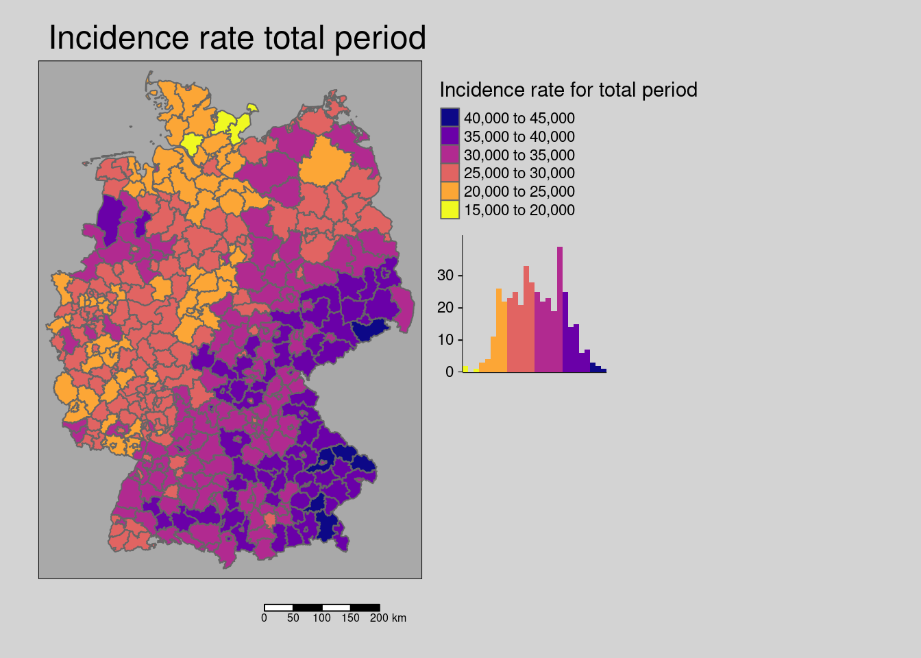
10.4.1.2 Share of foreigners
mForeigner <- covidKreise %>%
 tm_shape() +
  tm_polygons(col=c("Auslaenderanteil"),
              legend.hist = TRUE,
              legend.reverse = TRUE,
              title = "Share of foreigners of inhabitants [%]",
              style= "pretty") +
  tm_layout(legend.outside = TRUE, bg.color = "darkgrey",
            outer.bg.color = "lightgrey",
            legend.outside.size = 0.5, attr.outside = TRUE,
            main.title = "Foreign population") +
  tm_scale_bar()
## ## ── tmap v3 code detected ───────────────────────────────────────────────────────## [v3->v4] `tm_polygons()`: instead of `style = "pretty"`, use fill.scale =
## `tm_scale_intervals()`.
## ℹ Migrate the argument(s) 'style' to 'tm_scale_intervals(<HERE>)'
## [v3->v4] `tm_polygons()`: migrate the argument(s) related to the legend of the
## visual variable `fill` namely 'title', 'legend.reverse' (rename to 'reverse')
## to 'fill.legend = tm_legend(<HERE>)'
## [v3->v4] `tm_layout()`: use `tm_title()` instead of `tm_layout(main.title = )`
## ! `tm_scale_bar()` is deprecated. Please use `tm_scalebar()` instead.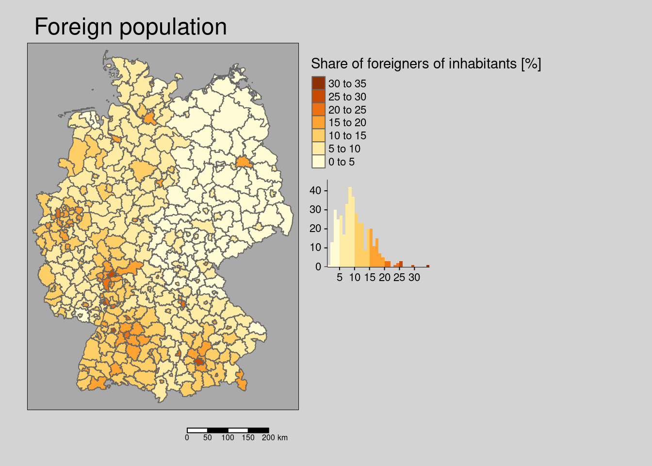
The share of foreigners at the population is spatially clustered as indicated by Moran’s I.
##
##  Monte-Carlo simulation of Moran I
##
## data:  covidKreise$Auslaenderanteil
## weights: unionedListw_d
## number of simulations + 1: 1000
##
## statistic = 0.46685, observed rank = 1000, p-value = 0.001
## alternative hypothesis: greater
The hypothesis is that the larger shares of foreigners indicate a larger share of inhabitants with limited skills in the German language a lower access to health and social distancing related information and that thereby districts with higher shares are associated with higher incidence rates.
10.4.1.3 Commuters
covidKreise %>%
tm_shape() +
  tm_polygons(col=c("Auspendler"),
              legend.hist = TRUE,
              legend.reverse = TRUE,
              title = "Outgoing commuters as share\nof total employees",
              style= "kmeans") +
  tm_layout(legend.outside = TRUE, bg.color = "darkgrey",
            outer.bg.color = "lightgrey",
            legend.outside.size = 0.5, attr.outside = TRUE,
            main.title = "Outgoing commuters") +
  tm_scale_bar()
## ## ── tmap v3 code detected ───────────────────────────────────────────────────────## [v3->v4] `tm_polygons()`: instead of `style = "kmeans"`, use fill.scale =
## `tm_scale_intervals()`.
## ℹ Migrate the argument(s) 'style' to 'tm_scale_intervals(<HERE>)'
## [v3->v4] `tm_polygons()`: migrate the argument(s) related to the legend of the
## visual variable `fill` namely 'title', 'legend.reverse' (rename to 'reverse')
## to 'fill.legend = tm_legend(<HERE>)'
## [v3->v4] `tm_layout()`: use `tm_title()` instead of `tm_layout(main.title = )`
## ! `tm_scale_bar()` is deprecated. Please use `tm_scalebar()` instead.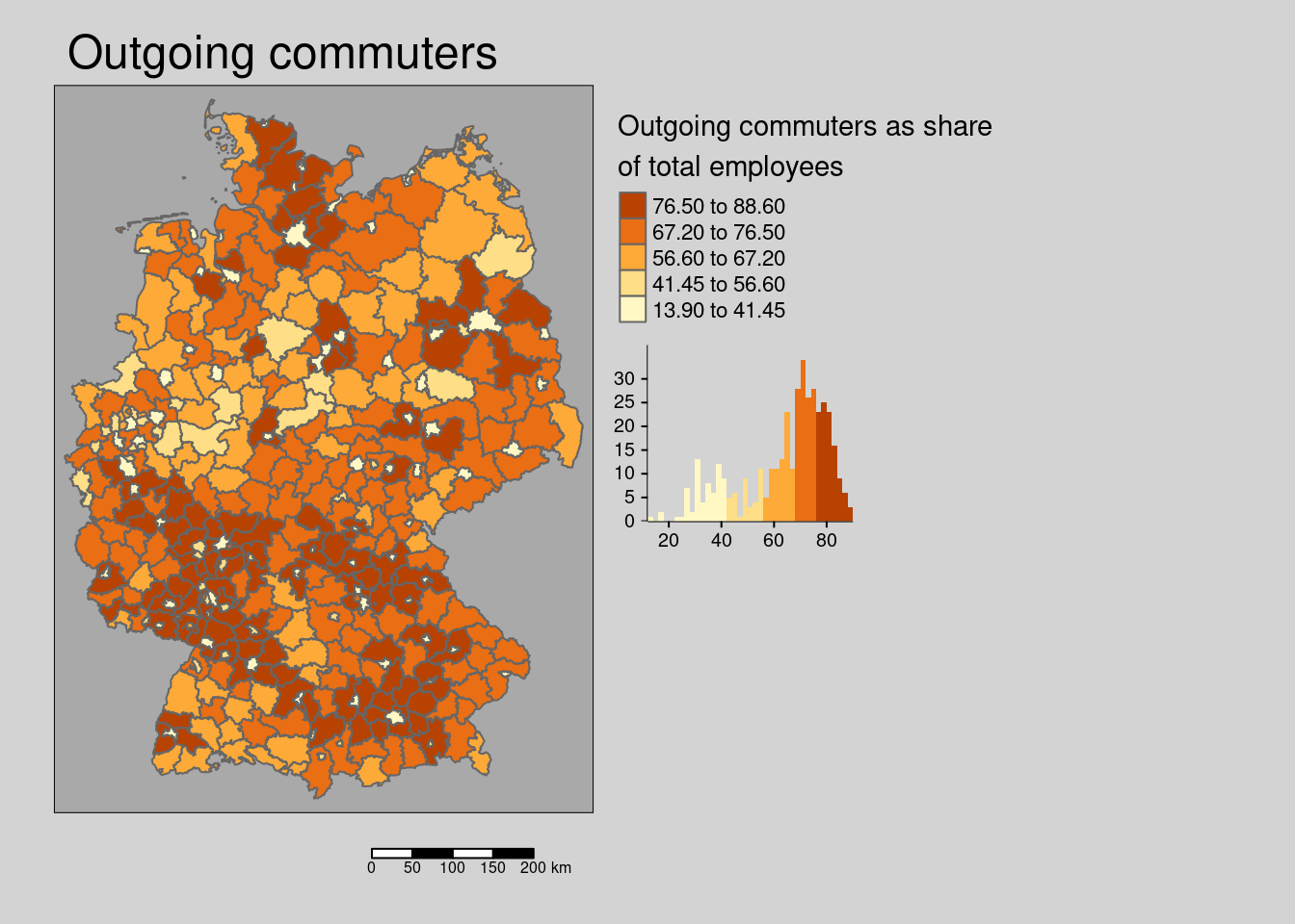
The share of outgoing commuter is randomly distributed in space.
##
##  Monte-Carlo simulation of Moran I
##
## data:  covidKreise$Auspendler
## weights: unionedListw_d
## number of simulations + 1: 1000
##
## statistic = -0.04866, observed rank = 10, p-value = 0.99
## alternative hypothesis: greater
covidKreise %>%
tm_shape() +
tm_polygons(col=c("Einpendler"),
legend.hist = TRUE,
legend.reverse = TRUE,
title = "Incoming commuters as share\nof total employees",
style= "kmeans") +
tm_layout(legend.outside = TRUE, bg.color = "darkgrey",
outer.bg.color = "lightgrey",
legend.outside.size = 0.5, attr.outside = TRUE,
main.title = "Incoming commuters") +
tm_scale_bar()## ## ── tmap v3 code detected ───────────────────────────────────────────────────────## [v3->v4] `tm_polygons()`: instead of `style = "kmeans"`, use fill.scale =
## `tm_scale_intervals()`.
## ℹ Migrate the argument(s) 'style' to 'tm_scale_intervals(<HERE>)'
## [v3->v4] `tm_polygons()`: migrate the argument(s) related to the legend of the
## visual variable `fill` namely 'title', 'legend.reverse' (rename to 'reverse')
## to 'fill.legend = tm_legend(<HERE>)'
## [v3->v4] `tm_layout()`: use `tm_title()` instead of `tm_layout(main.title = )`
## ! `tm_scale_bar()` is deprecated. Please use `tm_scalebar()` instead.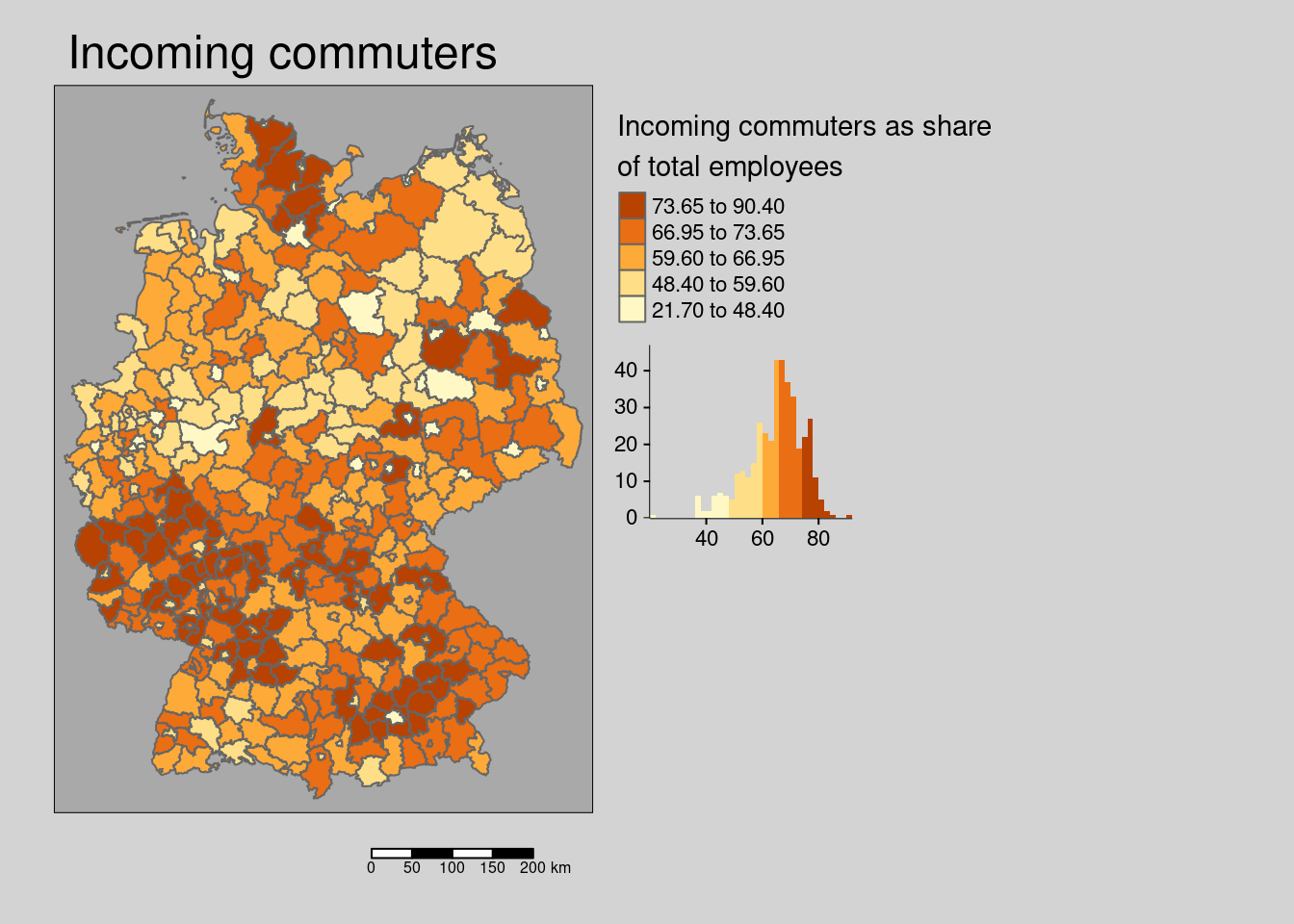
The share of incoming commuter is weakly clustered.
##
##  Monte-Carlo simulation of Moran I
##
## data:  covidKreise$Einpendler
## weights: unionedListw_d
## number of simulations + 1: 1000
##
## statistic = 0.23215, observed rank = 1000, p-value = 0.001
## alternative hypothesis: greater
The hypothesis for both incoming and outgoing commuters is that they indicate a spill-over of population between districts and thereby are associated with higher incidence rates.
10.4.1.4 Ruralness
mRural <- covidKreise %>%
 tm_shape() +
  tm_polygons(col=c("Laendlichkeit"),
              legend.hist = TRUE, palette = "Purples",
              legend.reverse = TRUE,
              title = "Share of inhabitants in places\nwith less then 150 Inh/sqkm",
              style= "kmeans") +
  tm_layout(legend.outside = TRUE, bg.color = "darkgrey",
            outer.bg.color = "lightgrey",
            legend.outside.size = 0.5, attr.outside = TRUE,
            main.title = "rurality") +
  tm_scale_bar()
## ## ── tmap v3 code detected ───────────────────────────────────────────────────────## [v3->v4] `tm_polygons()`: instead of `style = "kmeans"`, use fill.scale =
## `tm_scale_intervals()`.
## ℹ Migrate the argument(s) 'style', 'palette' (rename to 'values') to
## 'tm_scale_intervals(<HERE>)'
## [v3->v4] `tm_polygons()`: migrate the argument(s) related to the legend of the
## visual variable `fill` namely 'title', 'legend.reverse' (rename to 'reverse')
## to 'fill.legend = tm_legend(<HERE>)'
## [v3->v4] `tm_layout()`: use `tm_title()` instead of `tm_layout(main.title = )`
## ! `tm_scale_bar()` is deprecated. Please use `tm_scalebar()` instead.## [cols4all] color palettes: use palettes from the R package cols4all. Run
## `cols4all::c4a_gui()` to explore them. The old palette name "Purples" is named
## "brewer.purples"
## Multiple palettes called "purples" found: "brewer.purples", "matplotlib.purples". The first one, "brewer.purples", is returned.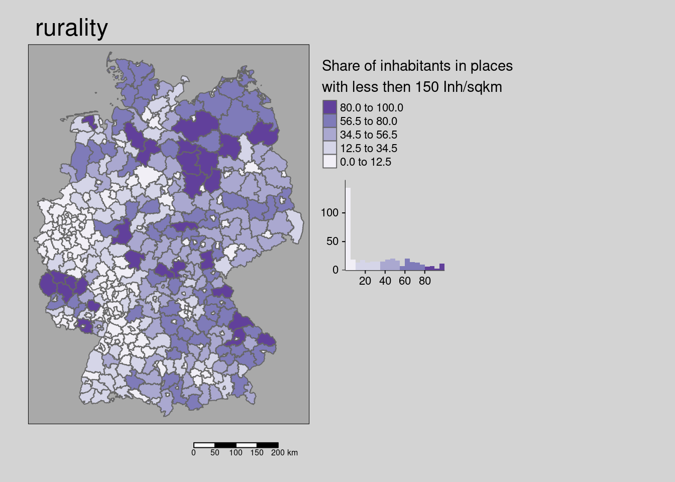
The share of inhabitants in places with less then 150 Inhabitants per sqkm is weakly spatially clustered.
##
## Monte-Carlo simulation of Moran I
##
## data: covidKreise$Laendlichkeit
## weights: unionedListw_d
## number of simulations + 1: 1000
##
## statistic = 0.22267, observed rank = 1000, p-value = 0.001
## alternative hypothesis: greaterThe hypothesis is that lower population densities and other modes of transport (less public transport) might lead to lower incidence rates.
10.4.1.5 Students
covidKreise %>%
tm_shape() +
tm_polygons(col=c("Studierende"),
legend.hist = TRUE, palette = "Purples",
legend.reverse = TRUE,
title = "Students per \n1000 Inhabitants",
style= "kmeans") +
tm_layout(legend.outside = TRUE, bg.color = "darkgrey",
outer.bg.color = "lightgrey",
legend.outside.size = 0.5, attr.outside = TRUE,
main.title = "Students") +
tm_scale_bar()## ## ── tmap v3 code detected ───────────────────────────────────────────────────────## [v3->v4] `tm_polygons()`: instead of `style = "kmeans"`, use fill.scale =
## `tm_scale_intervals()`.
## ℹ Migrate the argument(s) 'style', 'palette' (rename to 'values') to
## 'tm_scale_intervals(<HERE>)'
## [v3->v4] `tm_polygons()`: migrate the argument(s) related to the legend of the
## visual variable `fill` namely 'title', 'legend.reverse' (rename to 'reverse')
## to 'fill.legend = tm_legend(<HERE>)'
## [v3->v4] `tm_layout()`: use `tm_title()` instead of `tm_layout(main.title = )`
## ! `tm_scale_bar()` is deprecated. Please use `tm_scalebar()` instead.
## [cols4all] color palettes: use palettes from the R package cols4all. Run
## `cols4all::c4a_gui()` to explore them. The old palette name "Purples" is named
## "brewer.purples"
## Multiple palettes called "purples" found: "brewer.purples", "matplotlib.purples". The first one, "brewer.purples", is returned.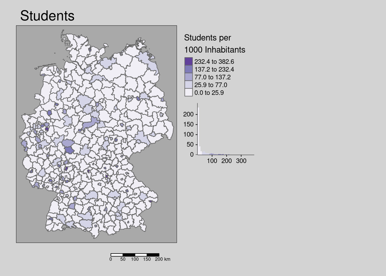
The number of students per 1000 inhabitants shows a very weak regular distribution pattern in space. Only a few districts host universities while neighboring districts often host only very limited numbers of students.
##
##  Monte-Carlo simulation of Moran I
##
## data:  covidKreise$Studierende
## weights: unionedListw_d
## number of simulations + 1: 1000
##
## statistic = -0.062607, observed rank = 1, p-value = 0.001
## alternative hypothesis: less
The hypothesis is that students have on average higher contact rates (under non-lockdown conditions) and also are spatially more mobile (moving between their living place and the town there their parents live for example) and districts with higher share of students might be associated with higher incidence rates.
10.4.1.6 Highly qualified workforce
covidKreise %>%
tm_shape() +
  tm_polygons(col=c("Hochqualifizierte"),
              legend.hist = TRUE,
              legend.reverse = TRUE,
              title = "Highly qualified employees/ total employees",
              style= "kmeans") +
  tm_layout(legend.outside = TRUE, bg.color = "darkgrey",
            outer.bg.color = "lightgrey",
            legend.outside.size = 0.5, attr.outside = TRUE,
            main.title = "Highly qualified employees") +
  tm_scale_bar()
## ## ── tmap v3 code detected ───────────────────────────────────────────────────────## [v3->v4] `tm_polygons()`: instead of `style = "kmeans"`, use fill.scale =
## `tm_scale_intervals()`.
## ℹ Migrate the argument(s) 'style' to 'tm_scale_intervals(<HERE>)'
## [v3->v4] `tm_polygons()`: migrate the argument(s) related to the legend of the
## visual variable `fill` namely 'title', 'legend.reverse' (rename to 'reverse')
## to 'fill.legend = tm_legend(<HERE>)'
## [v3->v4] `tm_layout()`: use `tm_title()` instead of `tm_layout(main.title = )`
## ! `tm_scale_bar()` is deprecated. Please use `tm_scalebar()` instead.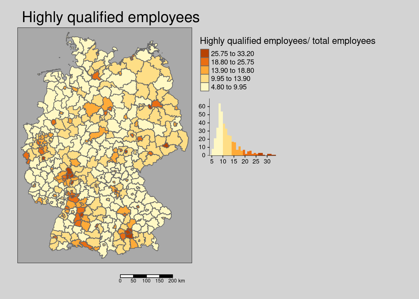
The share of highly qualified employees (employees with Bachelor or Master degree) is weakly spatially structured.
##
##  Monte-Carlo simulation of Moran I
##
## data:  covidKreise$Hochqualifizierte
## weights: unionedListw_d
## number of simulations + 1: 1000
##
## statistic = 0.16389, observed rank = 1000, p-value = 0.001
## alternative hypothesis: greater
The hypothesis is that employees with an academic degree more frequently work at home office and districts with a higher share are thereby associated with lower incidence rates.
10.4.1.7 Highspeed internet conncetivity
covidKreise %>%
tm_shape() +
  tm_polygons(col=c("Breitbandversorgung"),
              legend.hist = TRUE, palette = "Purples",
              legend.reverse = TRUE,
              title = "Share of households with internet \nconnectivity > 5 mBits/s",
              style= "kmeans") +
  tm_layout(legend.outside = TRUE, bg.color = "darkgrey", outer.bg.color = "lightgrey",
            legend.outside.size = 0.5, attr.outside = TRUE,
            main.title = "Highspeed internet") +
  tm_scale_bar()
## ## ── tmap v3 code detected ───────────────────────────────────────────────────────## [v3->v4] `tm_polygons()`: instead of `style = "kmeans"`, use fill.scale =
## `tm_scale_intervals()`.
## ℹ Migrate the argument(s) 'style', 'palette' (rename to 'values') to
## 'tm_scale_intervals(<HERE>)'
## [v3->v4] `tm_polygons()`: migrate the argument(s) related to the legend of the
## visual variable `fill` namely 'title', 'legend.reverse' (rename to 'reverse')
## to 'fill.legend = tm_legend(<HERE>)'
## [v3->v4] `tm_layout()`: use `tm_title()` instead of `tm_layout(main.title = )`
## ! `tm_scale_bar()` is deprecated. Please use `tm_scalebar()` instead.
## [cols4all] color palettes: use palettes from the R package cols4all. Run
## `cols4all::c4a_gui()` to explore them. The old palette name "Purples" is named
## "brewer.purples"
## Multiple palettes called "purples" found: "brewer.purples", "matplotlib.purples". The first one, "brewer.purples", is returned.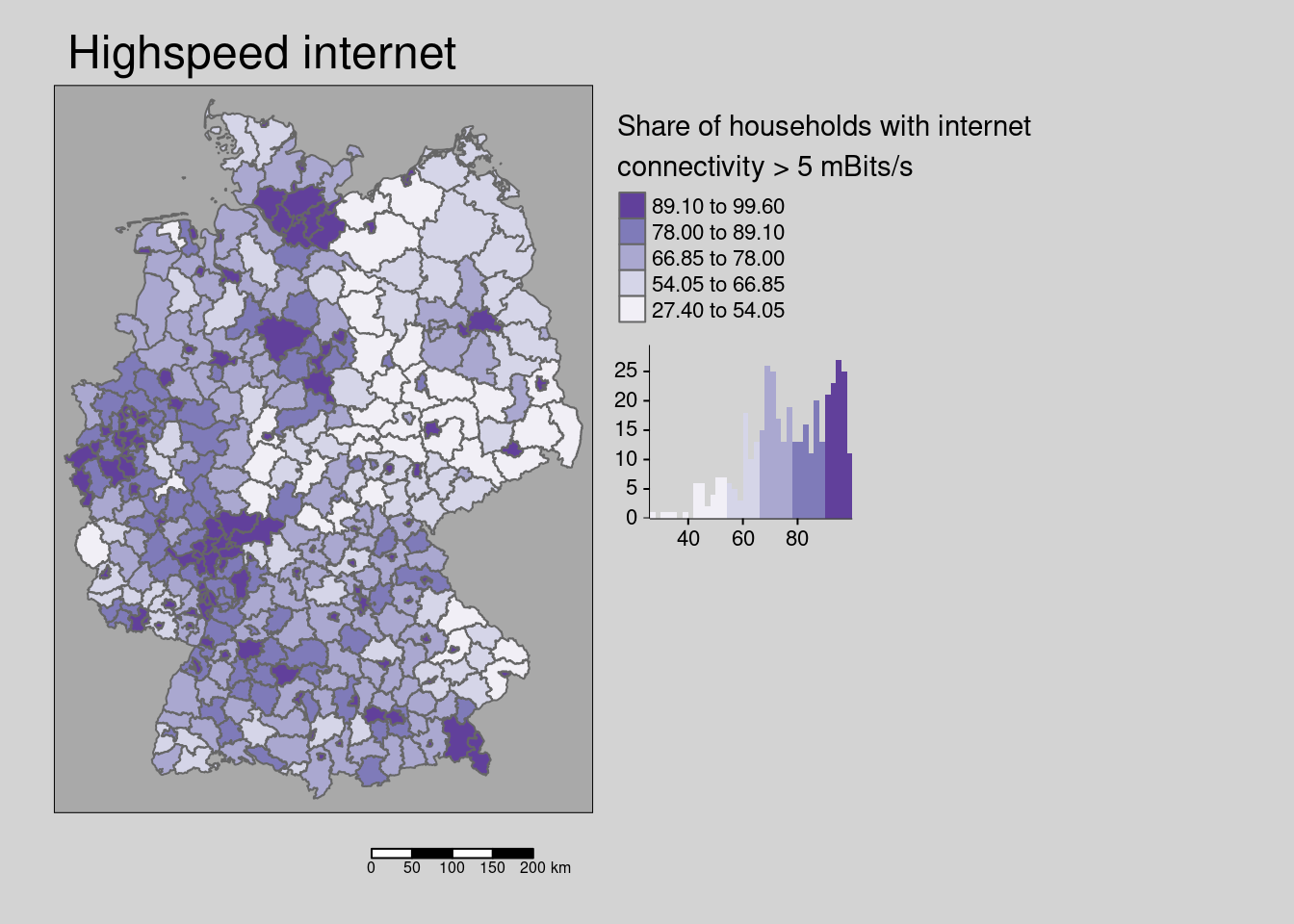
The share of households with internet connectivity greater than 5 mBits per second is weakly spatially structured.
##
##  Monte-Carlo simulation of Moran I
##
## data:  covidKreise$Breitbandversorgung
## weights: unionedListw_d
## number of simulations + 1: 1000
##
## statistic = 0.23278, observed rank = 1000, p-value = 0.001
## alternative hypothesis: greater
The hypothesis is that districts with better internet access offer higher potential for working in home office and thereby are associated with lower incidence rates.
10.4.1.8 Long term unemployment rate
covidKreise %>%
tm_shape() +
  tm_polygons(col=c("Langzeitarbeitslosenquote"),
              legend.hist = TRUE, palette="Oranges",
              legend.reverse = TRUE,
              title = "Unemployment rate [%]") +
  tm_layout(legend.outside = TRUE, bg.color = "darkgrey",
            outer.bg.color = "lightgrey",
            legend.outside.size = 0.5, attr.outside = TRUE,
            main.title = "Long term unemloyment rate") +
  tm_scale_bar()
## ## ── tmap v3 code detected ───────────────────────────────────────────────────────## [v3->v4] `tm_tm_polygons()`: migrate the argument(s) related to the scale of
## the visual variable `fill` namely 'palette' (rename to 'values') to fill.scale
## = tm_scale(<HERE>).
## [v3->v4] `tm_polygons()`: migrate the argument(s) related to the legend of the
## visual variable `fill` namely 'title', 'legend.reverse' (rename to 'reverse')
## to 'fill.legend = tm_legend(<HERE>)'
## [v3->v4] `tm_layout()`: use `tm_title()` instead of `tm_layout(main.title = )`
## ! `tm_scale_bar()` is deprecated. Please use `tm_scalebar()` instead.
## [cols4all] color palettes: use palettes from the R package cols4all. Run
## `cols4all::c4a_gui()` to explore them. The old palette name "Oranges" is named
## "brewer.oranges"
## Multiple palettes called "oranges" found: "brewer.oranges", "matplotlib.oranges". The first one, "brewer.oranges", is returned.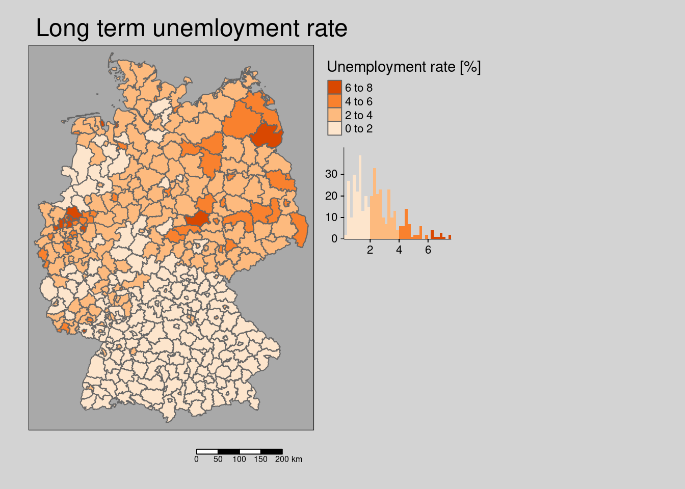
The long term unemployment rate is clearly spatially clustered.
##
##  Monte-Carlo simulation of Moran I
##
## data:  covidKreise$Langzeitarbeitslosenquote
## weights: unionedListw_d
## number of simulations + 1: 1000
##
## statistic = 0.59635, observed rank = 1000, p-value = 0.001
## alternative hypothesis: greater
The hypothesis is that the long term unemployment rate is associated with higher incidence rates as it is an indicator for economic conditions in general. Poorer districts might be facing higher incidence rates due to denser living conditions, less access to information and resources.
10.4.1.9 Right-winged votes
covidKreise %>%
tm_shape() +
  tm_polygons(col=c("Stimmenanteile.AfD"),
              legend.hist = TRUE, palette="Blues",
              legend.reverse = TRUE,
              title = "Share of votes at national election 2017") +
  tm_layout(legend.outside = TRUE, bg.color = "darkgrey",
            outer.bg.color = "lightgrey",
            legend.outside.size = 0.5, attr.outside = TRUE,
            main.title = "Right-winged party (AfD)") +
  tm_scale_bar()
## ## ── tmap v3 code detected ───────────────────────────────────────────────────────## [v3->v4] `tm_tm_polygons()`: migrate the argument(s) related to the scale of
## the visual variable `fill` namely 'palette' (rename to 'values') to fill.scale
## = tm_scale(<HERE>).
## [v3->v4] `tm_polygons()`: migrate the argument(s) related to the legend of the
## visual variable `fill` namely 'title', 'legend.reverse' (rename to 'reverse')
## to 'fill.legend = tm_legend(<HERE>)'
## [v3->v4] `tm_layout()`: use `tm_title()` instead of `tm_layout(main.title = )`
## ! `tm_scale_bar()` is deprecated. Please use `tm_scalebar()` instead.
## [cols4all] color palettes: use palettes from the R package cols4all. Run
## `cols4all::c4a_gui()` to explore them. The old palette name "Blues" is named
## "brewer.blues"
## Multiple palettes called "blues" found: "brewer.blues", "matplotlib.blues". The first one, "brewer.blues", is returned.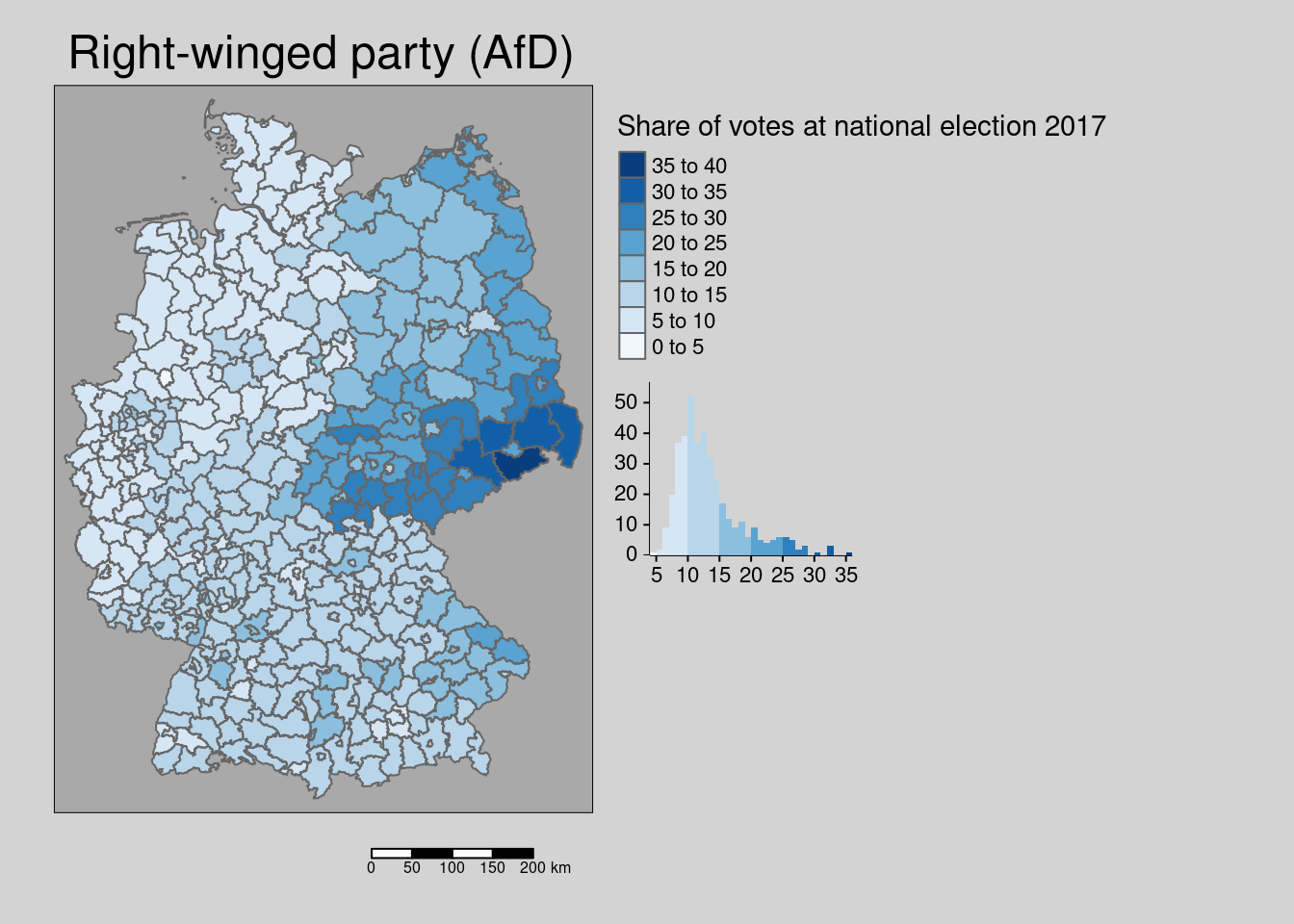
The share of votes for the biggest right-winged party (AfD) at the last election was clearly spatially clustered. The spatial distribution shows a clear east (former GDR)-west pattern with the the highest values in rural districts in Saxony.
##
##  Monte-Carlo simulation of Moran I
##
## data:  covidKreise$Stimmenanteile.AfD
## weights: unionedListw_d
## number of simulations + 1: 1000
##
## statistic = 0.73757, observed rank = 1000, p-value = 0.001
## alternative hypothesis: greater
The hypothesis is that the share of right-winged voters is a proxy for the share of the population skeptical with respect to social distancing, mask wearing and vaccination and might therefor be associated with higher incidence rates at the district level.
10.4.2 Scatterplot matrix
As a start we create a scatterplot matrix for the response and a number of potential predictors. For this plot we drop the sticky geometry columns and select the variables of interest. For the meaning of the variables and their units we refer to the choreplethe maps above.
st_drop_geometry(covidKreise) %>%
  dplyr::select(incidenceTotal, Langzeitarbeitslosenquote,
                Hochqualifizierte, Breitbandversorgung, Stimmenanteile.AfD,
                Studierende, Einpendler, Auspendler, Einpendler,
                Auslaenderanteil, Laendlichkeit) %>%
ggpairs(progress=FALSE) 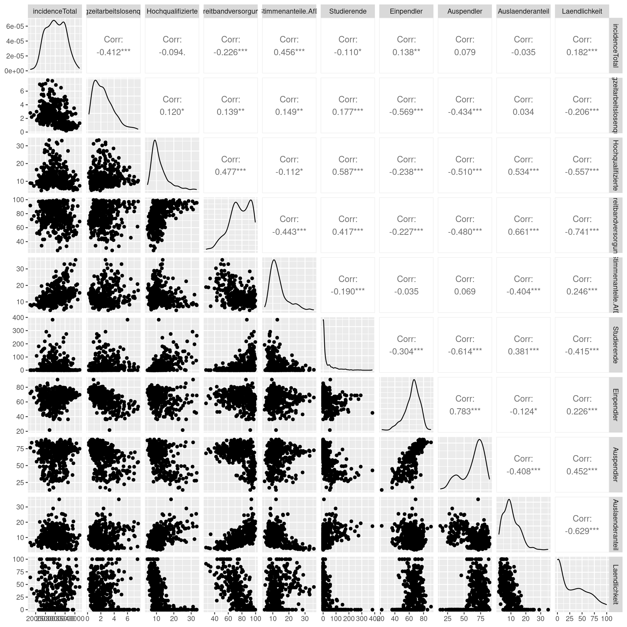
We see some predictors correlating with the incidence rate as well as some moderate collinearity between some of our predictors. We highlight a few observations and refer to the scatterplot matrix for further details.
The incidence rate is positively associated with the votes for the right-winged party and the share of foreigners at the district level. The long term unemployment rate is negatively associated with the share of outgoing and incoming commuters. The share of employees with an academic degree is positively associated with the availability of high-speed internet access, the number of students per population and the share of foreigners and negatively associated with the share of outgoing commuters and the share of the population living in rural areas. The share of votes for the right-winged party is negatively associated with the availability of highs-peed internet access and the share of foreigners. The share of foreigners is alo negatively associated with the rurality of the district. The share of students is negatively associated with the share of outgoing commuters. The availability of high-speed internet access is negatively associated with rurality, share of foreigners and the share of outgoing commutes and positively associated with the share of students.
10.4.3 Poisson GLM
We start with a normal GLM before checking for spatial autocorrelation in the residuals. Since we have count data a Poisson GLM with an offset for the population at risk seems a natural choice.
modelGlm <- glm(sumCasesTotal ~ Stimmenanteile.AfD + Auslaenderanteil + Hochqualifizierte + Langzeitarbeitslosenquote + Einpendler + Studierende + Laendlichkeit +  offset(log(EWZ)), data= covidKreise, family=poisson)
summary(modelGlm)
##
## Call:
## glm(formula = sumCasesTotal ~ Stimmenanteile.AfD + Auslaenderanteil +
## Hochqualifizierte + Langzeitarbeitslosenquote + Einpendler +
## Studierende + Laendlichkeit + offset(log(EWZ)), family = poisson,
## data = covidKreise)
##
## Coefficients:
## Estimate Std. Error z value Pr(>|z|)
## (Intercept) -1.264e+00 1.958e-03 -645.26 <2e-16 ***
## Stimmenanteile.AfD 1.788e-02 4.401e-05 406.23 <2e-16 ***
## Auslaenderanteil 9.064e-03 5.614e-05 161.44 <2e-16 ***
## Hochqualifizierte -4.523e-03 5.248e-05 -86.19 <2e-16 ***
## Langzeitarbeitslosenquote -5.572e-02 1.667e-04 -334.18 <2e-16 ***
## Einpendler -1.602e-03 1.891e-05 -84.70 <2e-16 ***
## Studierende 2.877e-04 5.327e-06 54.00 <2e-16 ***
## Laendlichkeit 4.751e-04 1.071e-05 44.35 <2e-16 ***
## ---
## Signif. codes: 0 '***' 0.001 '**' 0.01 '*' 0.05 '.' 0.1 ' ' 1
##
## (Dispersion parameter for poisson family taken to be 1)
##
## Null deviance: 555100 on 399 degrees of freedom
## Residual deviance: 276278 on 392 degrees of freedom
## AIC: 281340
##
## Number of Fisher Scoring iterations: 4Every regression coefficient estimated seems to be highly significant. However, we need to check for overdispersion as this might obscure uncertainty in the coefficient estimation.
10.4.4 Negative binomial GLM to account for overdispersion
Since we should be suspicious with respect to overdispersion we will run a negative binomial and afterwards a quasi-poisson GLM to account for that. Since the negative binomial GLM triggers some complications when using it with the spatial eigenvector mapping we will stay with the quasi-poisson model afterwards.
modelGlmNb <- glm.nb(sumCasesTotal ~ Stimmenanteile.AfD + Auslaenderanteil + Hochqualifizierte + Langzeitarbeitslosenquote + Einpendler + Studierende + Laendlichkeit + offset(log(EWZ)), data= covidKreise)
summary(modelGlmNb)
##
## Call:
## glm.nb(formula = sumCasesTotal ~ Stimmenanteile.AfD + Auslaenderanteil +
## Hochqualifizierte + Langzeitarbeitslosenquote + Einpendler +
## Studierende + Laendlichkeit + offset(log(EWZ)), data = covidKreise,
## init.theta = 77.61663303, link = log)
##
## Coefficients:
## Estimate Std. Error z value Pr(>|z|)
## (Intercept) -1.1952586 0.0633118 -18.879 < 2e-16 ***
## Stimmenanteile.AfD 0.0196991 0.0012106 16.273 < 2e-16 ***
## Auslaenderanteil 0.0109776 0.0015880 6.913 4.75e-12 ***
## Hochqualifizierte -0.0047725 0.0015737 -3.033 0.00242 **
## Langzeitarbeitslosenquote -0.0642848 0.0047604 -13.504 < 2e-16 ***
## Einpendler -0.0029401 0.0007166 -4.103 4.08e-05 ***
## Studierende 0.0001922 0.0001396 1.377 0.16865
## Laendlichkeit 0.0004701 0.0002654 1.771 0.07655 .
## ---
## Signif. codes: 0 '***' 0.001 '**' 0.01 '*' 0.05 '.' 0.1 ' ' 1
##
## (Dispersion parameter for Negative Binomial(77.6166) family taken to be 1)
##
## Null deviance: 826.01 on 399 degrees of freedom
## Residual deviance: 400.93 on 392 degrees of freedom
## AIC: 8036.2
##
## Number of Fisher Scoring iterations: 1
##
##
## Theta: 77.62
## Std. Err.: 5.49
##
## 2 x log-likelihood: -8018.193Considering overdisperion led to a serious increase in the standard errors. Two coefficients become insignificant as an effect. The general model selection strategy is that we should only drop on term at a time and not several together. We base our decision on the AIC and employ the drop1 convenience function which refits the model with single terms dropped - i.e. the model is refitted several times, each time on predictor is dropped from the start model. In our case we start with a model with 7 predictors, so drop1 fit 7 models with 6 predictors and reports the AIC. The model with the smallest AIC is preferable
## Single term deletions
##
## Model:
## sumCasesTotal ~ Stimmenanteile.AfD + Auslaenderanteil + Hochqualifizierte +
##     Langzeitarbeitslosenquote + Einpendler + Studierende + Laendlichkeit +
##     offset(log(EWZ))
##                           Df Deviance    AIC
## <none>                         400.93 8034.2
## Stimmenanteile.AfD         1   666.38 8297.6
## Auslaenderanteil           1   448.56 8079.8
## Hochqualifizierte          1   410.20 8041.5
## Langzeitarbeitslosenquote  1   584.55 8215.8
## Einpendler                 1   417.62 8048.9
## Studierende                1   402.85 8034.1
## Laendlichkeit              1   404.03 8035.3
Dropping ruralness seems beneficial as indicated by an AIC value higher than for the complete model (even if only slightly higher). We could reformulate the model or we could us the update function that allows us to add or drop terms from an existing model specification. The first argument is the model, the second the new formula: . indicates here all parts of the previous model, - Laendlichkeitindicates that the variable Laendlichkeitshould be dropped.
## Single term deletions
##
## Model:
## sumCasesTotal ~ Stimmenanteile.AfD + Auslaenderanteil + Hochqualifizierte +
##     Langzeitarbeitslosenquote + Einpendler + Studierende + offset(log(EWZ))
##                           Df Deviance    AIC
## <none>                         400.94 8035.3
## Stimmenanteile.AfD         1   669.82 8302.2
## Auslaenderanteil           1   447.00 8079.3
## Hochqualifizierte          1   414.03 8046.4
## Langzeitarbeitslosenquote  1   598.46 8230.8
## Einpendler                 1   417.44 8049.8
## Studierende                1   402.56 8034.9
The AIC decreases a bit if we drop the predictor share of students but as \(\Delta AIC\) is smaller than 2 we still decide to drop the predictor from the model.
##
## Call:
## glm.nb(formula = sumCasesTotal ~ Stimmenanteile.AfD + Auslaenderanteil +
##     Hochqualifizierte + Langzeitarbeitslosenquote + Einpendler +
##     offset(log(EWZ)), data = covidKreise, init.theta = 76.71067831,
##     link = log)
##
## Coefficients:
##                             Estimate Std. Error z value Pr(>|z|)
## (Intercept)               -1.1534361  0.0601197 -19.186  < 2e-16 ***
## Stimmenanteile.AfD         0.0196283  0.0012018  16.333  < 2e-16 ***
## Auslaenderanteil           0.0098194  0.0014408   6.815 9.40e-12 ***
## Hochqualifizierte         -0.0045761  0.0013450  -3.402 0.000668 ***
## Langzeitarbeitslosenquote -0.0655010  0.0047111 -13.903  < 2e-16 ***
## Einpendler                -0.0030835  0.0007115  -4.334 1.46e-05 ***
## ---
## Signif. codes:  0 '***' 0.001 '**' 0.01 '*' 0.05 '.' 0.1 ' ' 1
##
## (Dispersion parameter for Negative Binomial(76.7107) family taken to be 1)
##
##     Null deviance: 816.39  on 399  degrees of freedom
## Residual deviance: 400.94  on 394  degrees of freedom
## AIC: 8036.9
##
## Number of Fisher Scoring iterations: 1
##
##
##               Theta:  76.71
##           Std. Err.:  5.42
##
## 2 x log-likelihood: -8022.902## Single term deletions
##
## Model:
## sumCasesTotal ~ Stimmenanteile.AfD + Auslaenderanteil + Hochqualifizierte +
## Langzeitarbeitslosenquote + Einpendler + offset(log(EWZ))
## Df Deviance AIC
## <none> 400.94 8034.9
## Stimmenanteile.AfD 1 668.39 8300.4
## Auslaenderanteil 1 447.40 8079.4
## Hochqualifizierte 1 412.60 8044.6
## Langzeitarbeitslosenquote 1 596.42 8228.4
## Einpendler 1 419.50 8051.5AIC suggest to stay with that model.
10.4.5 Quasi-Poisson GLM to account for overdispersion
modelGlmQp <- glm(sumCasesTotal ~ Stimmenanteile.AfD + Auslaenderanteil + Hochqualifizierte + Langzeitarbeitslosenquote + Einpendler  + Studierende + Laendlichkeit + offset(log(EWZ)), data= covidKreise, family = quasipoisson)
summary(modelGlmQp)
##
## Call:
## glm(formula = sumCasesTotal ~ Stimmenanteile.AfD + Auslaenderanteil +
## Hochqualifizierte + Langzeitarbeitslosenquote + Einpendler +
## Studierende + Laendlichkeit + offset(log(EWZ)), family = quasipoisson,
## data = covidKreise)
##
## Coefficients:
## Estimate Std. Error t value Pr(>|t|)
## (Intercept) -1.2636569 0.0518225 -24.384 < 2e-16 ***
## Stimmenanteile.AfD 0.0178766 0.0011645 15.351 < 2e-16 ***
## Auslaenderanteil 0.0090642 0.0014857 6.101 2.53e-09 ***
## Hochqualifizierte -0.0045230 0.0013886 -3.257 0.00122 **
## Langzeitarbeitslosenquote -0.0557234 0.0044124 -12.629 < 2e-16 ***
## Einpendler -0.0016015 0.0005003 -3.201 0.00148 **
## Studierende 0.0002877 0.0001410 2.041 0.04196 *
## Laendlichkeit 0.0004751 0.0002834 1.676 0.09450 .
## ---
## Signif. codes: 0 '***' 0.001 '**' 0.01 '*' 0.05 '.' 0.1 ' ' 1
##
## (Dispersion parameter for quasipoisson family taken to be 700.2421)
##
## Null deviance: 555100 on 399 degrees of freedom
## Residual deviance: 276278 on 392 degrees of freedom
## AIC: NA
##
## Number of Fisher Scoring iterations: 4Strong overdispersion, as \(\phi\) has been estimated as 700.
## Single term deletions
##
## Model:
## sumCasesTotal ~ Stimmenanteile.AfD + Auslaenderanteil + Hochqualifizierte +
##     Langzeitarbeitslosenquote + Einpendler + Studierende + Laendlichkeit +
##     offset(log(EWZ))
##                           Df Deviance  F value    Pr(>F)
## <none>                         276278
## Stimmenanteile.AfD         1   437586 228.8744 < 2.2e-16 ***
## Auslaenderanteil           1   302131  36.6822 3.261e-09 ***
## Hochqualifizierte          1   283712  10.5487  0.001263 **
## Langzeitarbeitslosenquote  1   390350 161.8520 < 2.2e-16 ***
## Einpendler                 1   283440  10.1618  0.001549 **
## Studierende                1   279159   4.0885  0.043855 *
## Laendlichkeit              1   278241   2.7852  0.095939 .
## ---
## Signif. codes:  0 '***' 0.001 '**' 0.01 '*' 0.05 '.' 0.1 ' ' 1
The results of drop1tell us that the model that includes all six terms but not Laendlichkeit is only marginally significant different from the model with all seven parameters if we compare by deviance. In other words: the deviance increases a bit if we drop Laendlichkeit but not much. That means we get a smaller model that has the same quality of fit (measured by the deviance, the smaller the better). Following the principle of parsimony we would drop the term from the model.
## Single term deletions
##
## Model:
## sumCasesTotal ~ Stimmenanteile.AfD + Auslaenderanteil + Hochqualifizierte +
##     Langzeitarbeitslosenquote + Einpendler + Studierende + offset(log(EWZ))
##                           Df Deviance  F value    Pr(>F)
## <none>                         278241
## Stimmenanteile.AfD         1   446069 237.0480 < 2.2e-16 ***
## Auslaenderanteil           1   302207  33.8503 1.236e-08 ***
## Hochqualifizierte          1   288438  14.4034 0.0001708 ***
## Langzeitarbeitslosenquote  1   408979 184.6610 < 2.2e-16 ***
## Einpendler                 1   286086  11.0807 0.0009547 ***
## Studierende                1   280987   3.8787 0.0496052 *
## ---
## Signif. codes:  0 '***' 0.001 '**' 0.01 '*' 0.05 '.' 0.1 ' ' 1
The share of students is also marginally significant so we could think about dropping it. But we leave it for now.
Explained deviance:
## [1] 0.4987557##
## Call:
## glm(formula = sumCasesTotal ~ Stimmenanteile.AfD + Auslaenderanteil +
## Hochqualifizierte + Langzeitarbeitslosenquote + Einpendler +
## Studierende + offset(log(EWZ)), family = quasipoisson, data = covidKreise)
##
## Coefficients:
## Estimate Std. Error t value Pr(>|t|)
## (Intercept) -1.2290436 0.0476860 -25.774 < 2e-16 ***
## Stimmenanteile.AfD 0.0181074 0.0011595 15.617 < 2e-16 ***
## Auslaenderanteil 0.0082461 0.0014074 5.859 9.84e-09 ***
## Hochqualifizierte -0.0051201 0.0013462 -3.803 0.000165 ***
## Langzeitarbeitslosenquote -0.0576477 0.0042765 -13.480 < 2e-16 ***
## Einpendler -0.0016709 0.0005002 -3.340 0.000916 ***
## Studierende 0.0002805 0.0001412 1.986 0.047729 *
## ---
## Signif. codes: 0 '***' 0.001 '**' 0.01 '*' 0.05 '.' 0.1 ' ' 1
##
## (Dispersion parameter for quasipoisson family taken to be 704.3687)
##
## Null deviance: 555100 on 399 degrees of freedom
## Residual deviance: 278241 on 393 degrees of freedom
## AIC: NA
##
## Number of Fisher Scoring iterations: 4Explained deviance for the negative binomial GLM:
## [1] 0.5088874##
## Call:
## glm.nb(formula = sumCasesTotal ~ Stimmenanteile.AfD + Auslaenderanteil +
## Hochqualifizierte + Langzeitarbeitslosenquote + Einpendler +
## offset(log(EWZ)), data = covidKreise, init.theta = 76.71067831,
## link = log)
##
## Coefficients:
## Estimate Std. Error z value Pr(>|z|)
## (Intercept) -1.1534361 0.0601197 -19.186 < 2e-16 ***
## Stimmenanteile.AfD 0.0196283 0.0012018 16.333 < 2e-16 ***
## Auslaenderanteil 0.0098194 0.0014408 6.815 9.40e-12 ***
## Hochqualifizierte -0.0045761 0.0013450 -3.402 0.000668 ***
## Langzeitarbeitslosenquote -0.0655010 0.0047111 -13.903 < 2e-16 ***
## Einpendler -0.0030835 0.0007115 -4.334 1.46e-05 ***
## ---
## Signif. codes: 0 '***' 0.001 '**' 0.01 '*' 0.05 '.' 0.1 ' ' 1
##
## (Dispersion parameter for Negative Binomial(76.7107) family taken to be 1)
##
## Null deviance: 816.39 on 399 degrees of freedom
## Residual deviance: 400.94 on 394 degrees of freedom
## AIC: 8036.9
##
## Number of Fisher Scoring iterations: 1
##
##
## Theta: 76.71
## Std. Err.: 5.42
##
## 2 x log-likelihood: -8022.902We end up with two models of decent quality. Directions of effect seem to be aligned with expectations:
- higher share of votes for right winged party is associated with higher incidence (both models). Presumably a proxy for the share of population opposing mask wearing and social distancing and vaccination
- higher share of foreigners is associated with higher incidence (both models). Foreigners might not be reach by information campaigns with respect to social distancing due to language problems
- higher share of highly qualified work force is associated with lower incidence rates (both models). For those employees it might be easier to work from home office and to avoid close contacts during work hours at office.
- higher long term unemployment rates were associated with lower incidence rates in both models. This is not what we expected. The map above shows that the lowest long term unemployment rates are in Bavaria and Baden-Württemberg with partialy very high incidence rates.
- higher rates of incomming commuters were associated with lower incidence rates. This also is not in line with our hypothesis.
##               (Intercept)        Stimmenanteile.AfD          Auslaenderanteil
##             -1.2290435997              0.0181073660              0.0082460642
##         Hochqualifizierte Langzeitarbeitslosenquote                Einpendler
##             -0.0051200895             -0.0576477446             -0.0016708665
##               Studierende
## 0.0002804845## (Intercept) Stimmenanteile.AfD Auslaenderanteil
## -1.153436063 0.019628305 0.009819398
## Hochqualifizierte Langzeitarbeitslosenquote Einpendler
## -0.004576117 -0.065500955 -0.00308353810.4.6 Effect plots for both NB and QP model
I demonstrate here we use of two conveneint functions to create predition plots. These help to better understand the model behavior. The ggpredict function has the additional opportunity to add partial residuals to the plot.
10.4.6.1 Using sjPlot
We can use convenience function e.g from the sjPlot package to plot the behaviour of the models. If we specify type="pred" we get plots of the estimated relationship between each predictor and the response at the response scale (already back transformed). In addition the estimated confidence bands are provided.
require(sjPlot)

pAfD_qp <- plot_model(modelGlmQp, type="pred",
           terms=c("Stimmenanteile.AfD"),
           condition = c(EWZ =  10^5)) +
  labs(title="Predicted COVID-19 cases",
       subtitle="Quasi-Poisson GLM for 100,000 inh.") +
  xlab("Share of votes for the right winged party AfD") +
  ylab("COVID-19 cases")

plUenemp_qp <-plot_model(modelGlmQp, type="pred",
           terms=c("Langzeitarbeitslosenquote"),
           condition = c(EWZ =  10^5)) +
  labs(title="Predicted COVID-19 cases",
       subtitle="Quasi-Poisson GLM for 100,000 inh.") +
  xlab("Long term unemployment rate") +
  ylab("COVID-19 cases")

ggarrange(pAfD_qp, plUenemp_qp)
And for the selected model for the negative binomial GLM:
pAfD_nb <-plot_model(modelGlmNb, type="pred",
           terms=c("Stimmenanteile.AfD"),
           condition = c(EWZ =  10^5)) +
  labs(title="Predicted COVID-19 cases",
       subtitle="Negative Binomial GLM  for 100,000 inh.") +
  xlab("Share of votes for the right winged party AfD") +
  ylab("COVID-19 cases")

plUenemp_nb <- plot_model(modelGlmNb, type="pred",
           terms=c("Langzeitarbeitslosenquote"),
           condition = c(EWZ =  10^5)) +
  labs(title="Predicted COVID-19 cases",
       subtitle="Negative Binomial GLM for 100,000 inh.") +
  xlab("Long term unemployment rate") +
  ylab("COVID-19 cases")

ggarrange(pAfD_qp, plUenemp_qp,
          pAfD_nb, plUenemp_nb)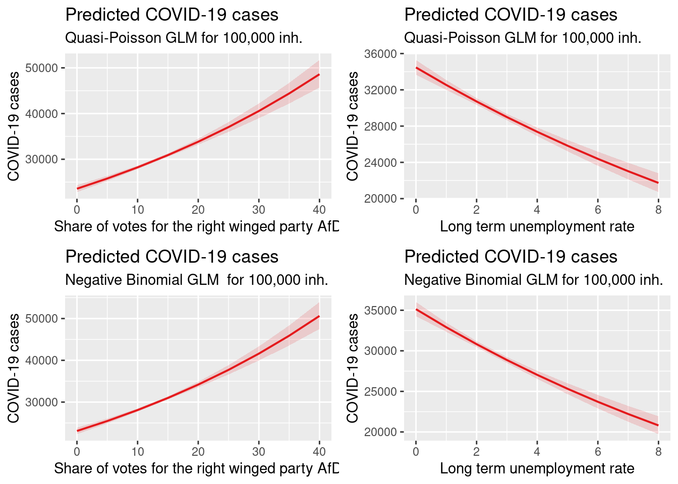
10.4.6.2 Using ggpredict
We will use ggpredict from the ggeffect package to create effect plots. The plots created are always partial residual plots - i.e. adjusted for the effect of the other predictors in the model.
p1 <- ggpredict(modelGlmNb, terms = "Stimmenanteile.AfD[all]",
                condition = c(EWZ = 10^5)) %>%
  plot(show_residuals=TRUE, jitter= TRUE) + labs(title =  "NB, 100,000 inh.") +
  xlab("Share votes right-winged [%]") + ylab("COVID-19 cases")
p2 <- ggpredict(modelGlmQp, terms = "Stimmenanteile.AfD[all]",
                condition = c(EWZ = 10^5)) %>%
  plot(show_residuals=TRUE, jitter=TRUE) + labs(title =  "QP, 100,000 inh.")+
  xlab("Share votes right-winged [%]") + ylab("COVID-19 cases")

ggarrange(p1,p2)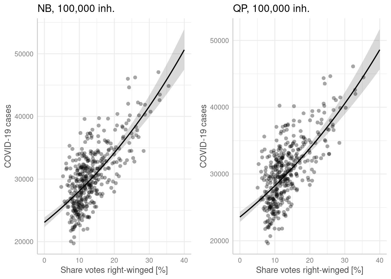
p1 <- ggpredict(modelGlmNb, terms = "Auslaenderanteil[all]",
                condition = c(EWZ = 10^5)) %>%
  plot(show_residuals=TRUE, jitter=TRUE) + labs(title =  "NB, 100,000 inh.") +
  xlab("Share foreigners [%]") + ylab("COVID-19 cases")
p2 <- ggpredict(modelGlmQp, terms = "Auslaenderanteil[all]",
                condition = c(EWZ = 10^5)) %>%
  plot(show_residuals=TRUE, jitter=TRUE) + labs(title =  "QP, 100,000 inh.")+
  xlab("Share foreigners [%]") + ylab("COVID-19 cases")

ggarrange(p1,p2)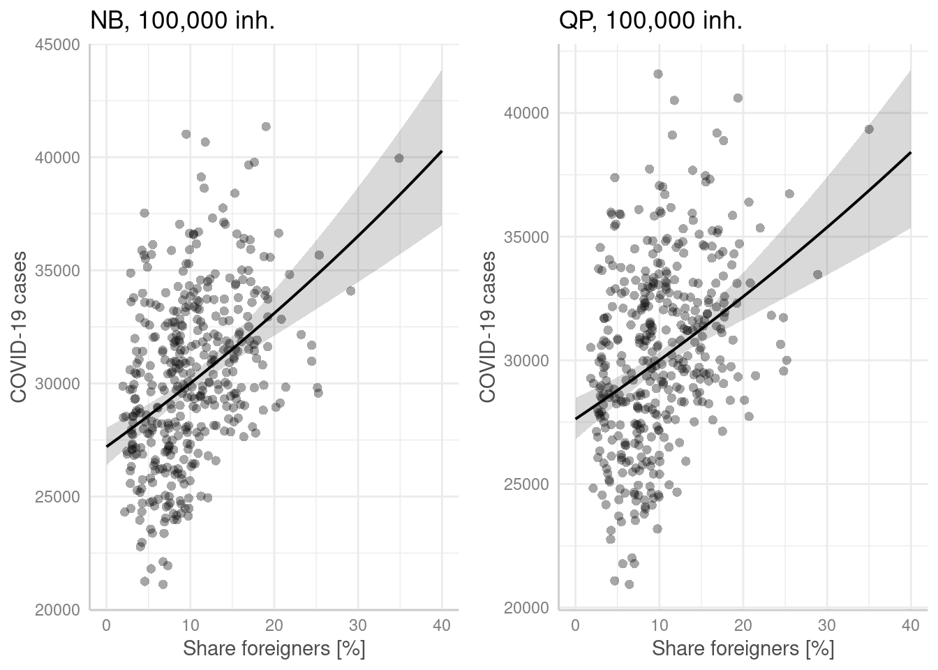
p1 <- ggpredict(modelGlmNb, terms = "Hochqualifizierte[all]",
                condition = c(EWZ = 10^5)) %>%
  plot(show_residuals=TRUE, jitter=TRUE) + labs(title =  "NB, 100,000 inh.") +
  xlab("Share highly qualified jobs [%]") + ylab("COVID-19 cases")
p2 <- ggpredict(modelGlmQp, terms = "Hochqualifizierte[all]",
                condition = c(EWZ = 10^5)) %>%
  plot(show_residuals=TRUE, jitter=TRUE) + labs(title =  "QP, 100,000 inh.")+
  xlab("Share highly qualified jobs [%]") + ylab("COVID-19 cases")

ggarrange(p1,p2)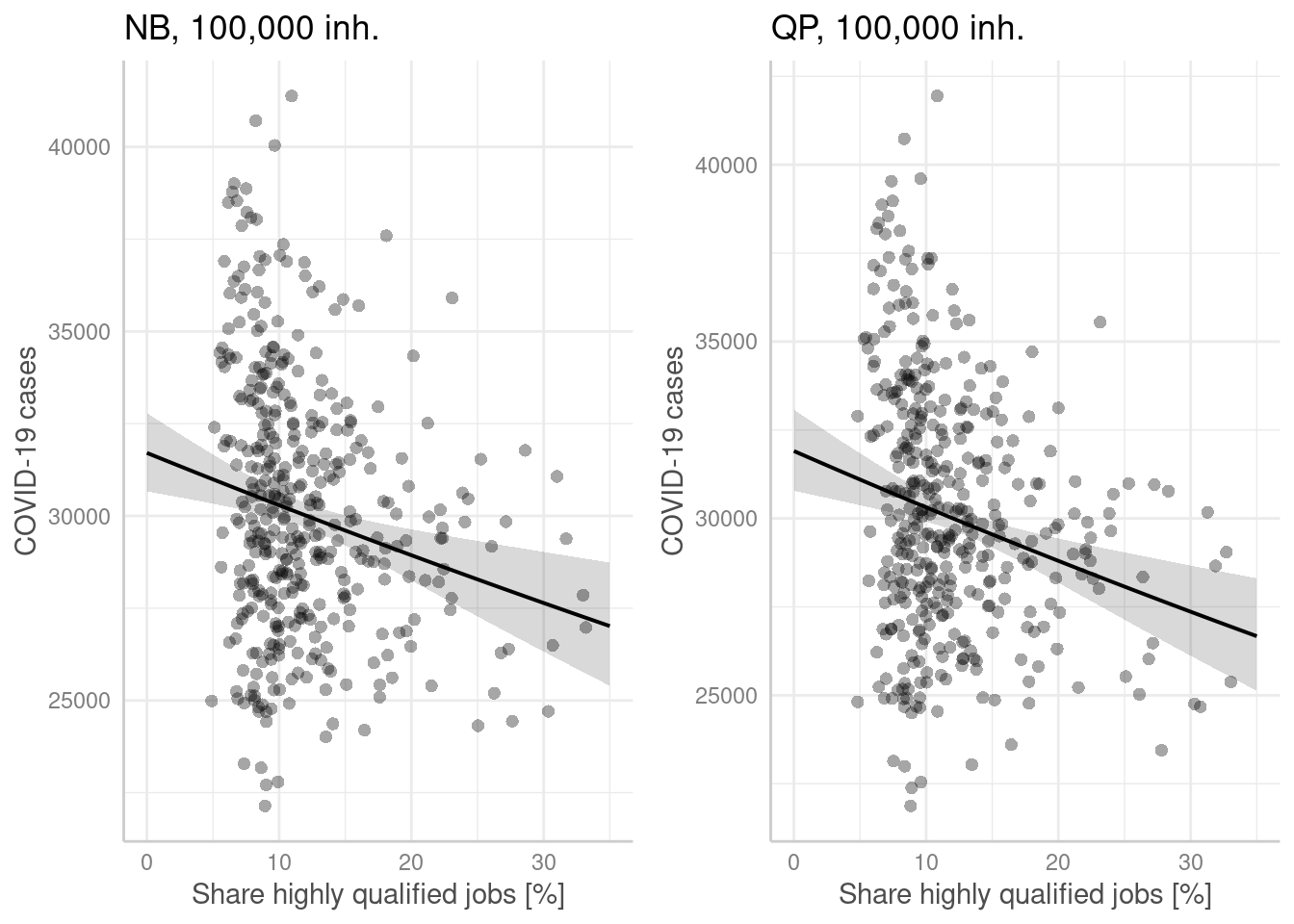
p1 <- ggpredict(modelGlmNb, terms = "Einpendler[all]",
                condition = c(EWZ = 10^5)) %>%
  plot(show_residuals=TRUE, jitter=TRUE) + labs(title =  "NB, 100,000 inh.") +
  xlab("Share incomming commuters on total jobs [%]") + ylab("COVID-19 cases")
p2 <- ggpredict(modelGlmQp, terms = "Einpendler[all]",
                condition = c(EWZ = 10^5)) %>%
  plot(show_residuals=TRUE, jitter=TRUE) + labs(title =  "QP, 100,000 inh.")+
  xlab("Share incomming commuters on total jobs [%]") + ylab("COVID-19 cases")

ggarrange(p1,p2)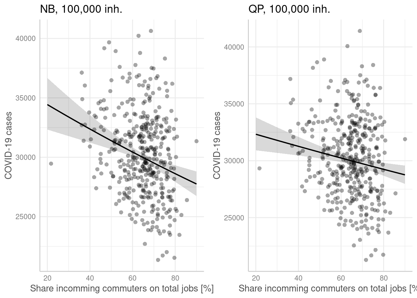
p1 <- ggpredict(modelGlmNb, terms = "Langzeitarbeitslosenquote[all]",
                condition = c(EWZ = 10^5)) %>%
  plot(show_residuals=TRUE, jitter=TRUE) + labs(title =  "NB, 100,000 inh.") +
  xlab("Longterm unemployment rate [%]") + ylab("COVID-19 cases")
p2 <- ggpredict(modelGlmQp, terms = "Langzeitarbeitslosenquote[all]",
                condition = c(EWZ = 10^5)) %>%
  plot(show_residuals=TRUE, jitter=TRUE) + labs(title =  "QP, 100,000 inh.")+
  xlab("Longterm unemployment rate [%]") + ylab("COVID-19 cases")

ggarrange(p1,p2)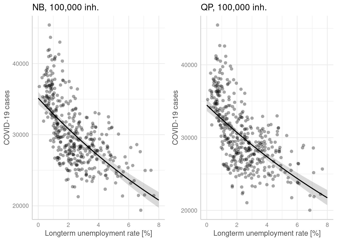
For the negative binomial GLM we have dropped the number of students per 1000 inhabitatns. Therefore, we only show one plot for this predictor.
ggpredict(modelGlmQp, terms = "Studierende[all]",
          condition=c(EWZ=10^5)) %>%
  plot(show_residuals=TRUE) + labs(title =  "QP, 100,000 inh.")+
  xlab("Students per 1000 inh.") + ylab("COVID-19 cases")
## Data points may overlap. Use the `jitter` argument to add some amount of
## random variation to the location of data points and avoid overplotting.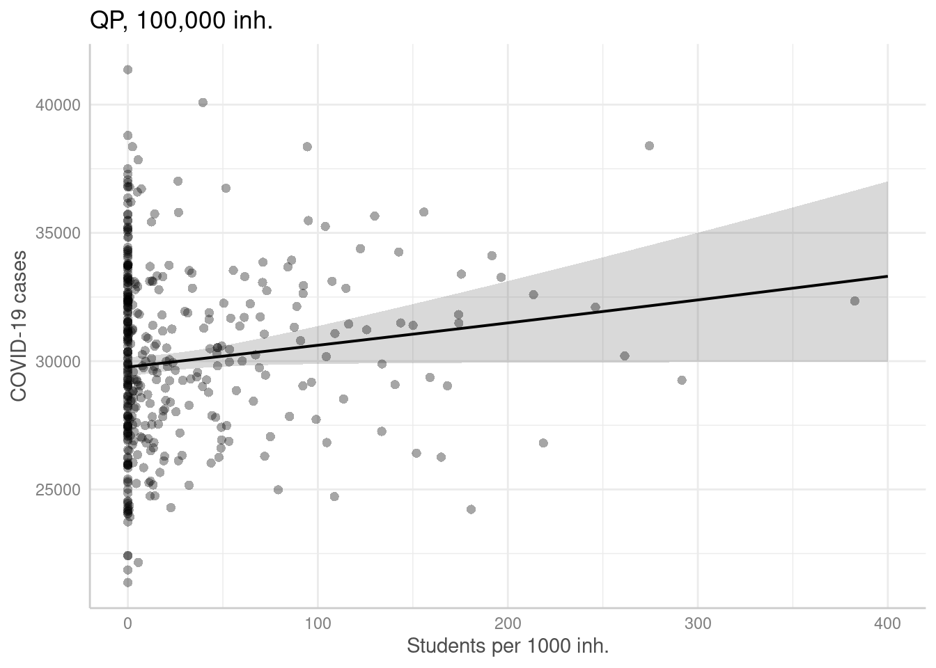
10.4.7 Checking for spatial autocorrelation in the residuals
10.4.7.1 Global Moran’s I
For regression residuals we need to use a different test as residuals are centered around zero and will sum up to zero.
##
##  Global Moran I for regression residuals
##
## data:
## model: glm.nb(formula = sumCasesTotal ~ Stimmenanteile.AfD +
## Auslaenderanteil + Hochqualifizierte + Langzeitarbeitslosenquote +
## Einpendler + offset(log(EWZ)), data = covidKreise, init.theta =
## 76.71067831, link = log)
## weights: unionedListw_d
##
## Moran I statistic standard deviate = 17.785, p-value < 2.2e-16
## alternative hypothesis: greater
## sample estimates:
## Observed Moran I      Expectation         Variance
## 0.3690786338 -0.0001015050 0.0004308865##
## Global Moran I for regression residuals
##
## data:
## model: glm(formula = sumCasesTotal ~ Stimmenanteile.AfD +
## Auslaenderanteil + Hochqualifizierte + Langzeitarbeitslosenquote +
## Einpendler + Studierende + offset(log(EWZ)), family = quasipoisson,
## data = covidKreise)
## weights: unionedListw_d
##
## Moran I statistic standard deviate = 17.52, p-value < 2.2e-16
## alternative hypothesis: greater
## sample estimates:
## Observed Moran I Expectation Variance
## 3.650420e-01 -1.295453e-07 4.341364e-04Both model suffer from significant global spatial autocorrelation.
This implies that the usual assumption about independence of errors is violated. In turn, our standard errors might be too low, p-values too small, size (and potentially even sign) of the regression coefficients might be wrong. So we need to incorporate spatial autocorrelation in our analysis. We will approach this by means of spatial eigenvector mapping.
10.4.7.2 Plot residuals
First we create centroids that we use in turn for a proportional symbol map of the residuals.
## Warning: st_point_on_surface assumes attributes are constant over geometriesAdd residuals to the centroids for plotting. In addition to the (deviance) residuals we also store their absolute values as this is need to scale the symbols.
kreisePoS$residGlmNb <- residuals(modelGlmNb)
kreisePoS$residGlmNbAbs <- abs(kreisePoS$residGlmNb)

kreisePoS$residGlmQp <- residuals(modelGlmQp)
kreisePoS$residGlmQpAbs <- abs(kreisePoS$residGlmQp)
The size of the symbols is taken from the absolute value while the color is assigned based on the deviance residuals.
# col= "residGlmNb", palette = "-RdBu",
             # alpha=.9, perceptual=TRUE, scale=.8, border.alpha=.3,
             # title.size = "Abs residual", title.col="Residuals", n=3
m1 <- tm_shape(covidKreise) +
  tm_polygons(fill="grey") +
  tm_shape(kreisePoS) +
  tm_bubbles( fill="residGlmNb",
              fill.scale= tm_scale_intervals(values=  "-brewer.rd_bu", midpoint=0),
              fill_alpha =.8,
              fill.legend= tm_legend(title = "Residuals",
                                                reverse=TRUE),
             size = "residGlmNbAbs",
             size.legend= tm_legend(title= "Abs. residuals"),
             size.scale = tm_scale_intervals(n=3)
             ) +
  tm_layout(legend.outside = TRUE, attr.outside = TRUE) +
    tm_title("Pearson residuals, GLM NB") +
   tm_scalebar()


m2 <- tm_shape(covidKreise) +
  tm_polygons(col="grey") +
  tm_shape(kreisePoS) +
  tm_bubbles( fill="residGlmQp",
              fill.scale= tm_scale_intervals(values=  "-brewer.rd_bu", midpoint=0),
              fill_alpha =.8,
              fill.legend= tm_legend(title = "Residuals",
                                                reverse=TRUE),
             size = "residGlmNbAbs",
             size.legend= tm_legend(title= "Abs. residuals"),
             size.scale = tm_scale_intervals(n=3)
             ) +
  tm_layout(legend.outside = TRUE, attr.outside = TRUE) +
    tm_title("Pearson residuals, GLM QP") +
   tm_scalebar()

tmap_arrange(m1,m2)
## [plot mode] fit legend/component: Some legend items or map compoments do not
## fit well, and are therefore rescaled.
## ℹ Set the tmap option `component.autoscale = FALSE` to disable rescaling.
## [plot mode] fit legend/component: Some legend items or map compoments do not
## fit well, and are therefore rescaled.
## ℹ Set the tmap option `component.autoscale = FALSE` to disable rescaling.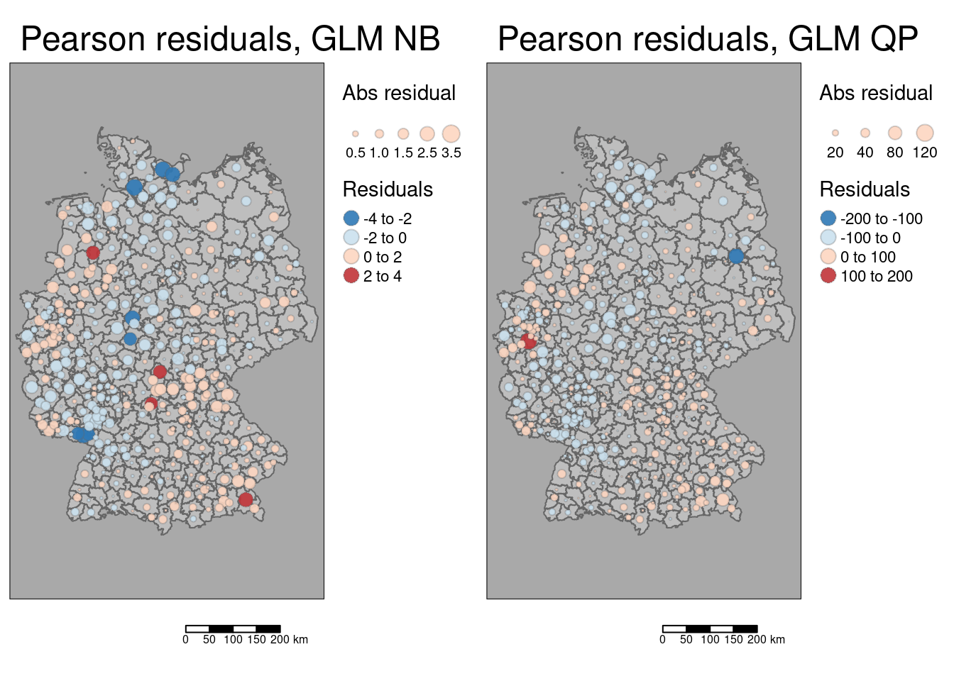
As indicated by global Moran’s I we see that large positive and large negative residuals form some cluster. The higher complexity of the quasi-poisson GLM leads to smaller residuals for some districts.
10.5 Recommended reading
(Dunn and Smyth, 2018) provide an excellent and accessible overview about generalized linear models in R.
References
The name of this distribution comes from applying the binomial theorem with a negative exponent.↩︎