Chapter 11 Spatial explorative data analysis - geographically weighted regression
require(spgwr)
require(sf)
require(tmap)
require(tidyverse)
require(ggplot2)
require(GGally)
require(corrplot)
require(ggpubr)
11.1 Cheat sheet
The following packages are used in this section:
ggwr- on of several packages that offers GWR functionality, here selected as it offers the feature to use generalized linear models in addition to linear modelssftmaptidyverseggplot2GGally- for a ggplot2 scatter plot matrixcorrplot- for nice polts of correlation matrices
Important commands:
spgwr::ggwr- fitting a generalized linear GWR modelspgwr::ggwr.sel- selecting a bandwidth or an adaptive kernel size for a generalized linear GWR model
11.2 Theory
The geographically weighted regression (GWR) (Brunsdon et al., 2000) (Ali et al., 2007) is an explorative tool that is shaky for hypothesis testing. So it should not be mistaken as a proper regression analysis.
It is a local approach that fits a regression model for each subset of the dataset (c.f. figure 11.1). Subsets are defined either based on a fixed distance or on k-nearest neighbors (adaptive) (Guo et al., 2008). The best neighborhood for a dataset is selected in a cross-validation approach. One can think of the approach as of a focal function with a window moving across the study region, always selecting the part of the data that is inside the distance band or that fulfills the k-nearest neighbor criteria. Based on that subset a regression model is fitted and coefficients and standard errors (not for GLM) stored for the i-th spatial object. As the regression is fitted \(n\) times for \(n\) data points (spatial objects) we end up with \(n\) sets of regression coefficients. If these coefficients vary across space this can be taken as an indication that we are missing a spatially distributed factor in our regression model. This factor might be a missing co-variate or a missing interaction or a truly auto-correlative process.
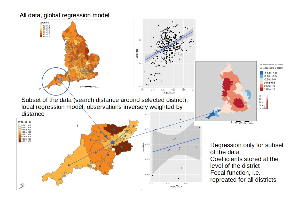
Figure 11.1: Geographically weighted regression
While a linear model has a common set of coefficients fitted to all data this is different for the GWR. For the GWR a separate model is fitted for each spatial unit, always using a different subset.
Linear model:
\[y = \beta_0 + \beta_1 x_1 + \beta_2 x_2 + ... \beta_n x_n + \epsilon\] \[\epsilon \sim N(0, \sigma)\] Linear GWR model:
\[y_i = \beta_{0i} + \beta_{1i} x_{1i} + \beta_{2i} x_{2i} + ... \beta_{ni} x_{ni} + \epsilon_i\] \[\epsilon_i \sim N(0, \sigma)\] This implies, that for each spatial unit (e.g. district) a separate regression model is fitted. This also implies that we have separate regression coefficients for each spatial unit. This allows us to study if effects are varying in space and provides us potentially hints for interpretation.
Observations are thereby downweighted according to distance. Three different kernels are implemented for this weighting, from which the tricube kernel is not available for GLM type GWRs.
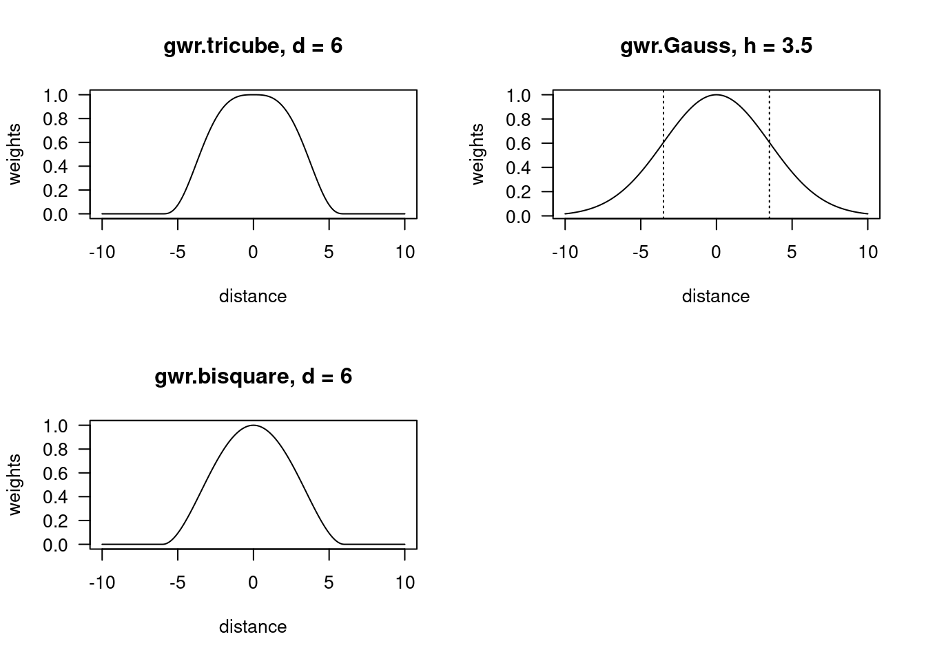
The equations are as follows:
- gaussian kernel: \(w_{i,j}(g) = e^{-(\frac{d_{i,j}}{h})^2 }\)
- bisquare kernel: \(w_{i,j}(g) = (1-\frac{d_{i,j}^3}{d^3})^3\) if \(d_{i,j}\leq d\) and \(w_{i,j}(g)=0\) everywhere else
- tricube kernel: \(w_{i,j}(g) = (1-\frac{d_{i,j}^2}{d^2})^2\) if \(d_{i,j}\leq d\) and \(w_{i,j}(g)=0\) everywhere else
with \(d_{i,j}\) the distances between the observations \(i\) and \(j\) and \(h\) the bandwidth.
For the bisquare and the tricube kernel the weights approach zero at distance \(d\). This implies a discontinuity in space. The exponential function used for the gaussian kernel converges againt zero for \(\pm \infty\) but never reaches 0. That implies that continuity in space is assumed - even far away points have some influence.
In the narrower sense, bandwidth is only defined for the gaussian kernel, for the other two kernels \(d\) is estimated which has a different meaning.
One thing to keep in mind then using GWR is the problem of multicollinearity between the coefficient estimates - even if the predictors them self are not collinear (Wheeler and Tiefelsdorf, 2005).
The ggwr command allows us to run generalized linear models in the context of the gwr.
\[ g(y_i) = \beta_{0i} + \beta_{1i} x_{1i} + \beta_{2i} x_{2i} + ... \beta_{ni} x_{ni} \] In case of the Poisson GLM:
\[ y_i \tilde{} P(\lambda)\] The bandwidth selection procedure fits the GWR several times with different bandwidth settings. Each time a local regression is fitted to all data points inside the bandwidth - however, the data point at the location for which the local regression is fitted is left out. This means, the model is only fitted the neighboring observations, but not the observation in focus. Now, the difference between the predicted and the observed response value is calculated squared (squared CV error). The sum of all squared CV errors across all observations is used the the objective that should be minimized. An optimization approach is used for the minimization, that uses a combination of golden section search and successive parabolic interpolation.
For linear GWR models the selection of the bandwidth by means of the AIC is the preferred approach. Unfortunately, this option is not available for GLM GWR in spgwr.
Hint: A general warning is to not blindly rely on the estimated optimal bandwidth. The approach is prune to the influence of outliers does not consider situations were the different predictors in the model work at different scales. Some more advanced selection procedures have been proposed Farber and Páez (2007) but are not available in spgwr and beyond scope here. It is advisable to check for the sum of weights to identify areas without much neighbors (especially for the fixed bandwidth models), especially if the spatial units are of very different size. Smaller bandwidths tend to increase the variability of the coefficients across space.
11.3 COVID-19 case study
Here we only need the district layer and not the neighborhood definition as GWR is only using euclidian distance (at least in the spgwr package). The spgwr function currently requires input in sp format. Therefore, we convert the sf object to a SpatialPolygonsDataFrame.
covidKreise <- st_read(dsn = "data/covidKreise.gpkg", layer = "kreiseWithCovidMeldeWeeklyCleaned", quiet=TRUE)
covidKreiseSp <- as(covidKreise, "Spatial")
11.3.1 Fitting GWR models
11.3.1.1 Adaptive bandwidth (based on the number of points)
We first estimate the optimal number of points to be included in the local regression - however, this is needs a bit of time. ggwr.sel uses a cross-validation approach to find the best value and returns it. The function fits the GWR several times with different bandwidth settings. Each time a local regression is fitted to all data points inside the bandwidth - however, the data point at the location for which the local regression is fitted is left out. This means, the model is only fitted the neighboring observations, but not the observation in focus. Now, the difference between the predicted and the observed response value is calculated squared (squared CV error). The the sum of all squared CV errors across all observations is used the the objective that should be minimized (if parameter RSME=FALSE is set, which is the default). An optimization approach is used for the minimization, that uses a combination of golden section search and successive parabolic interpolation.
adaptPerc <- ggwr.sel(sumCasesTotal ~ Stimmenanteile.AfD +
                        Auslaenderanteil + Hochqualifizierte +
                        Langzeitarbeitslosenquote + Einpendler  +
                        Studierende + Laendlichkeit + offset(log(EWZ)),
                        adapt = TRUE,family = "quasipoisson", data = covidKreiseSp)
## Adaptive q: 0.381966 CV score: 58828299426
## Adaptive q: 0.618034 CV score: 61056924284
## Adaptive q: 0.236068 CV score: 55654671781
## Adaptive q: 0.145898 CV score: 53733686027
## Adaptive q: 0.09016994 CV score: 55201579006
## Adaptive q: 0.158364 CV score: 53923445759
## Adaptive q: 0.139643 CV score: 53626712624
## Adaptive q: 0.120746 CV score: 53973215179
## Adaptive q: 0.132425 CV score: 53673060547
## Adaptive q: 0.1378729 CV score: 53657069048
## Adaptive q: 0.1420322 CV score: 53686210788
## Adaptive q: 0.1405556 CV score: 53638549324
## Adaptive q: 0.1395217 CV score: 53628622058
## Adaptive q: 0.1398657 CV score: 53623272321
## Adaptive q: 0.1401293 CV score: 53625234776
## Adaptive q: 0.1399184 CV score: 53622470963
## Adaptive q: 0.1399629 CV score: 53621798386
## Adaptive q: 0.1400264 CV score: 53622053879
## Adaptive q: 0.1399629 CV score: 53621798386## Selected adaptive bandwidth (% observations): 14%.If you would be up to using the bandwidth suggested by ggwr.sel you could just use the value returned by it, which represents the faction of all data points (if adapt = TRUE has been specified, otherwise it would be a distance in map units), i.e. ggwr(…., adapt = adaptPerc,…)).
gGwrAdaptPo <- ggwr(sumCasesTotal ~ Stimmenanteile.AfD +
                        Auslaenderanteil + Hochqualifizierte +
                        Langzeitarbeitslosenquote + Einpendler  +
                        Studierende + Laendlichkeit + offset(log(EWZ)),
                    family = "quasipoisson", data = covidKreiseSp, adapt=adaptPerc, type="deviance")
print(gGwrAdaptPo)
## Call:
## ggwr(formula = sumCasesTotal ~ Stimmenanteile.AfD + Auslaenderanteil +
## Hochqualifizierte + Langzeitarbeitslosenquote + Einpendler +
## Studierende + Laendlichkeit + offset(log(EWZ)), data = covidKreiseSp,
## adapt = adaptPerc, family = "quasipoisson", type = "deviance")
## Kernel function: gwr.Gauss
## Adaptive quantile: 0.1399629 (about 55 of 400 data points)
## Summary of GWR coefficient estimates at data points:
## Min. 1st Qu. Median 3rd Qu.
## X.Intercept. -1.4407e+00 -1.2505e+00 -1.0604e+00 -9.8525e-01
## Stimmenanteile.AfD 3.7625e-03 1.3020e-02 1.4028e-02 1.7684e-02
## Auslaenderanteil 2.3491e-03 4.4101e-03 5.9403e-03 8.5169e-03
## Hochqualifizierte -1.0258e-02 -4.5302e-03 -3.2536e-03 -2.0241e-03
## Langzeitarbeitslosenquote -8.5906e-02 -7.0792e-02 -5.3670e-02 -4.6852e-02
## Einpendler -4.9964e-03 -4.5094e-03 -3.2534e-03 -1.9427e-03
## Studierende -1.7671e-04 -2.0460e-05 1.2020e-04 2.6348e-04
## Laendlichkeit -5.3658e-04 -1.8636e-04 1.6383e-04 6.8977e-04
## Max. Global
## X.Intercept. -9.1362e-01 -1.2637
## Stimmenanteile.AfD 2.2281e-02 0.0179
## Auslaenderanteil 1.6765e-02 0.0091
## Hochqualifizierte 2.1026e-03 -0.0045
## Langzeitarbeitslosenquote -3.4980e-02 -0.0557
## Einpendler -9.4361e-05 -0.0016
## Studierende 5.7467e-04 0.0003
## Laendlichkeit 1.3157e-03 0.0005We see that the coefficients for most predictors vary by a good order of magnitude and do not change their sign for the adaptive kernel width chosen. However, there are three exceptions for which we observe a change in the direction of the effect (the sign): - the share of students (Studierende) - rurality (Laendlichkeit) - share of highly qualified employees (Hochqualifizierte)
The coefficients are stored in the SDF slot of the spgwr object. This is a SpatialPolygonsDatanFrame that stores the regression coefficients, the dispersion parameter if quasi-family distribution are used and the residuals.
## Object of class SpatialPolygonsDataFrame
## Coordinates:
##         min       max
## x  280371.1  921292.4
## y 5235856.0 6101443.7
## Is projected: TRUE
## proj4string :
## [+proj=utm +zone=32 +ellps=GRS80 +towgs84=0,0,0,0,0,0,0 +units=m
## +no_defs]
## Data attributes:
##      sum.w         X.Intercept.     Stimmenanteile.AfD Auslaenderanteil
##  Min.   : 72.58   Min.   :-1.4407   Min.   :0.003763   Min.   :0.002349
##  1st Qu.: 86.86   1st Qu.:-1.2505   1st Qu.:0.013020   1st Qu.:0.004410
##  Median : 92.84   Median :-1.0604   Median :0.014028   Median :0.005940
##  Mean   : 93.99   Mean   :-1.1159   Mean   :0.014575   Mean   :0.006818
##  3rd Qu.: 98.79   3rd Qu.:-0.9852   3rd Qu.:0.017684   3rd Qu.:0.008517
##  Max.   :129.98   Max.   :-0.9136   Max.   :0.022281   Max.   :0.016765
##  Hochqualifizierte   Langzeitarbeitslosenquote   Einpendler
##  Min.   :-0.010258   Min.   :-0.08591          Min.   :-4.996e-03
##  1st Qu.:-0.004530   1st Qu.:-0.07079          1st Qu.:-4.509e-03
##  Median :-0.003254   Median :-0.05367          Median :-3.253e-03
##  Mean   :-0.003412   Mean   :-0.05775          Mean   :-3.036e-03
##  3rd Qu.:-0.002024   3rd Qu.:-0.04685          3rd Qu.:-1.943e-03
##  Max.   : 0.002103   Max.   :-0.03498          Max.   :-9.436e-05
##   Studierende         Laendlichkeit          dispersion     deviance_resids
##  Min.   :-1.767e-04   Min.   :-0.0005366   Min.   : 47.05   Min.   :-70.9818
##  1st Qu.:-2.046e-05   1st Qu.:-0.0001864   1st Qu.: 94.93   1st Qu.:-13.6186
##  Median : 1.202e-04   Median : 0.0001638   Median :131.07   Median : -0.4757
##  Mean   : 1.353e-04   Mean   : 0.0002828   Mean   :133.36   Mean   : -1.1933
##  3rd Qu.: 2.635e-04   3rd Qu.: 0.0006898   3rd Qu.:168.41   3rd Qu.: 11.2404
##  Max.   : 5.747e-04   Max.   : 0.0013157   Max.   :226.86   Max.   : 62.9413
Lets plot the distibution of the coefficient estimates by histograms:
globalLm <-data.frame(coefficients(gGwrAdaptPo$lm))
names(globalLm) <- "Coefficient.global"
globalLm$Predictor <- row.names(globalLm)
idx <- which(globalLm$Predictor == "(Intercept)")
globalLm$Predictor[idx] <- "X.Intercept."
globalLm$type <- "Global"


gGwrAdaptPo$SDF %>% as.data.frame() %>%
  dplyr::select(X.Intercept.:Laendlichkeit) %>%
  pivot_longer(cols = everything(), names_to = "Predictor",
               values_to = "Coefficient") %>%
  ggplot(mapping= aes(x=Coefficient)) + geom_histogram(bins=50) +
  geom_vline(mapping = aes(xintercept = 0, color = "zero"), lty = 2, show.legend=TRUE)  +
  facet_wrap(~ Predictor, scales = "free") +
  geom_vline(aes(xintercept= Coefficient.global, color="global"), data=globalLm, lty=2, show.legend=TRUE) +
  scale_color_manual(name = "Reference",
                     values= c(zero = "blue", global = "red"))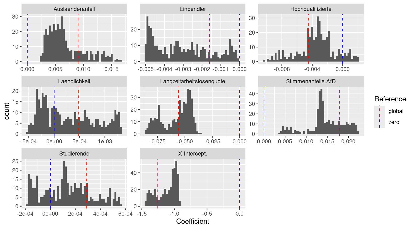
Now lets plot maps of the regression coefficients to get an overview about how they vary in space. Please keep in mind that we do get neither p-values nor standard errors for the GWR-regression coefficients.
tmap_mode("plot")

# convert sp to sf
gGwrAdaptPo_sf <- st_as_sf(gGwrAdaptPo$SDF)

m1 <- tm_shape(gGwrAdaptPo_sf) +
  tm_fill(fill="Stimmenanteile.AfD",
          fill.legend = tm_legend(title = "Coef. for right winged voters", reverse=TRUE),
          fill.scale = tm_scale_intervals(values = "brewer.reds", n=7)
          ) +
  tm_layout(legend.outside = TRUE, bg="lightgrey", attr.outside = TRUE)+
  tm_scalebar() +
  tm_title("GWR regression coefficients, adaptive")

mAfd <- tm_shape(covidKreise) +
  tm_fill(fill="Stimmenanteile.AfD",
          fill.legend = tm_legend(title = "Share right winged voters", reverse=TRUE),
          fill.scale= tm_scale_intervals(values = "brewer.blues", n=7)
        ) +
  tm_layout(legend.outside = TRUE, bg="lightgrey", attr.outside = TRUE)+
  tm_scalebar() +
  tm_title("INKAR data")

tmap_arrange(m1, mAfd)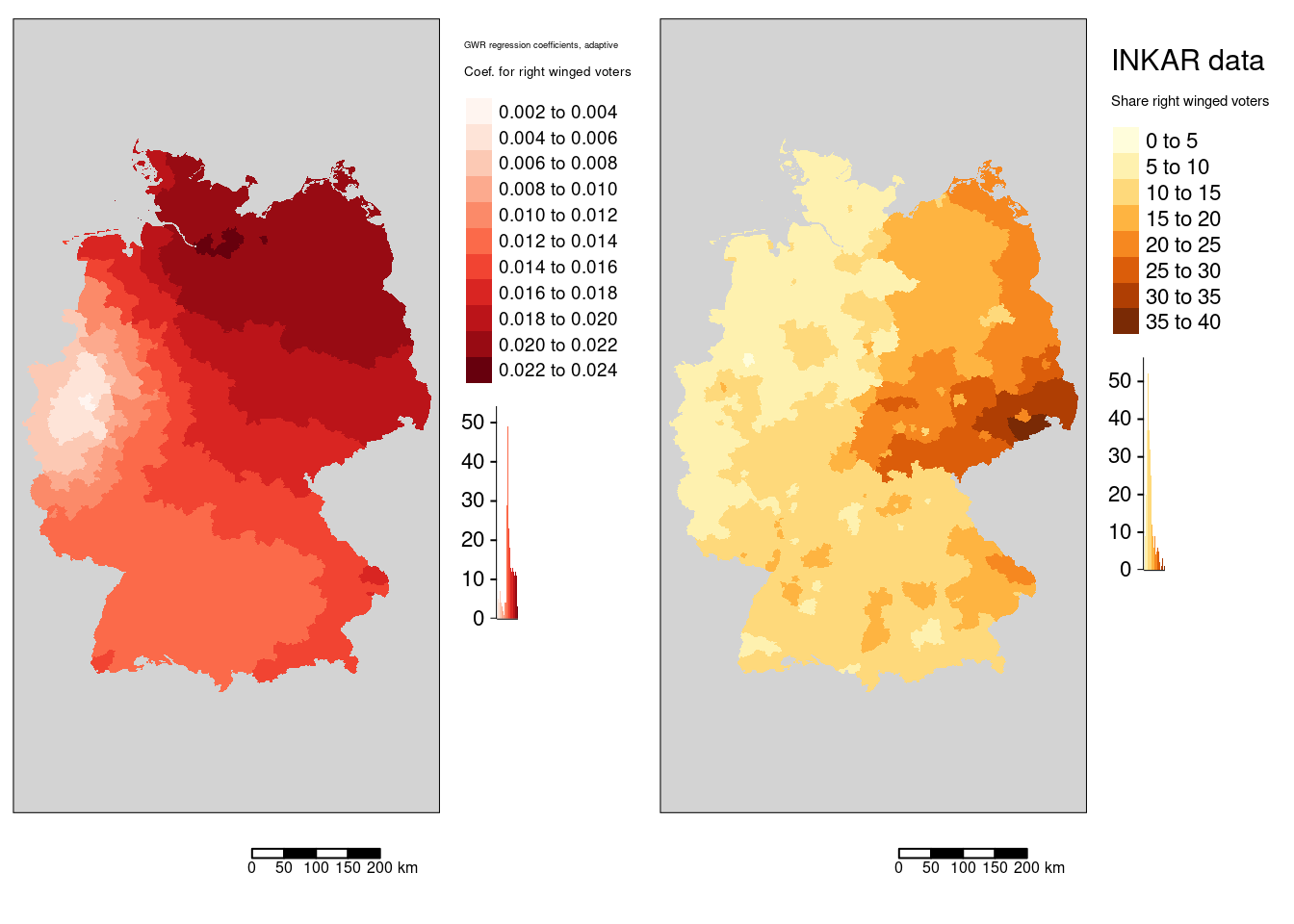
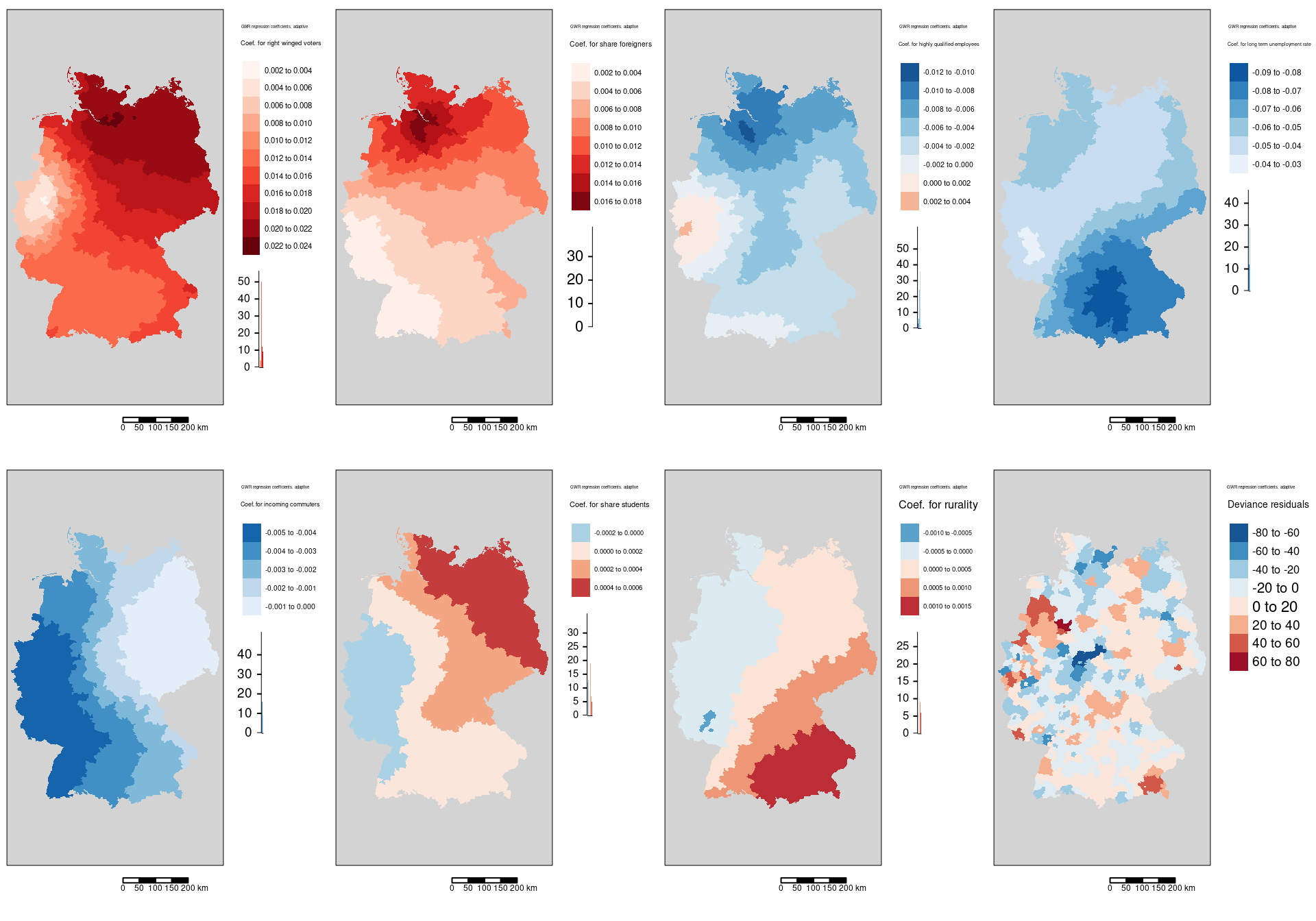
We see that the regression coefficient for the percentage of votes for the far right was positively associated with the covid-19 rate and that the effect was strongest in Hamburg, Meckelenburg-Vorpommern and Schleswig-Holstein. The lowest association was observed in the districts around the Ruhrgebiet - the weakest association was found for the Ennepe-Ruhr-Kreis. The general spatial pattern indicates a weakening association from north-east to sout-west with the western part of NRW as a region with outstandingly low association.
For interpretation we have to combine the spatially varying regression coefficients with the predictor. As we are using a GLM with the log-link we have to use the following formula (cf. 10:
\[\text{effect_j} = (e^{\beta_j})^{x_{i,j}}\] where \(i\) is the i-th predictor (here votes for the right winged party) and \(j\) is the index of the location.
covidKreise$Stimmenanteile.AfD_effect <- exp(gGwrAdaptPo$SDF$Stimmenanteile.AfD) ^covidKreise$Stimmenanteile.AfD

tm_shape(covidKreise) +
  tm_fill(fill="Stimmenanteile.AfD_effect",
          fill.chart = tm_chart_histogram(),
          fill.legend= tm_legend(title = "Effect right winged voters", reverse=TRUE),
          fill.scale= tm_scale_intervals(values = "brewer.purples" , n=7)) +
  tm_layout(legend.outside = TRUE, bg="lightgrey", attr.outside = TRUE)+
  tm_scalebar() + tm_title("Predictor effect GWR, adaptive")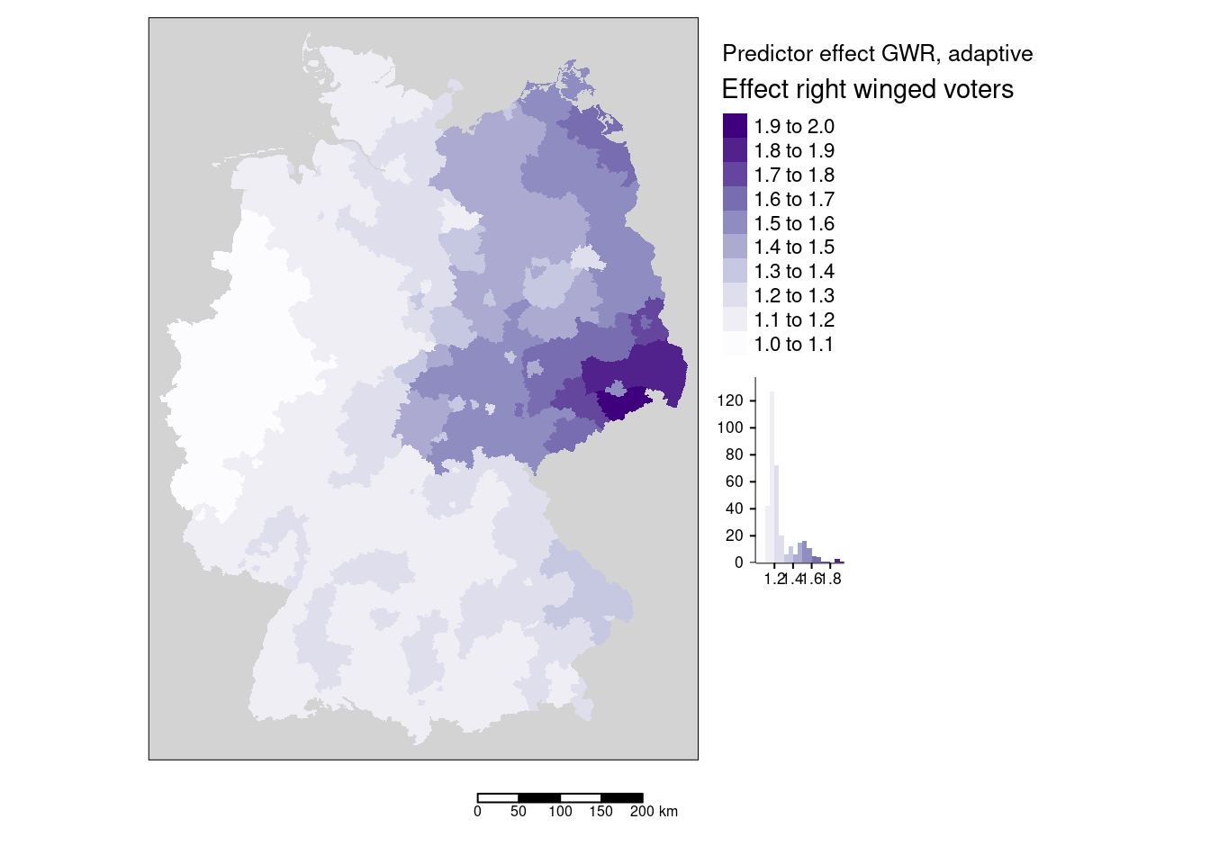
This value would then be multiplied by the spatially varying intercept.
covidKreise$Stimmenanteile.AfD_effectTimesInterc <- exp(gGwrAdaptPo$SDF$X.Intercept.)* covidKreise$Stimmenanteile.AfD_effect

tm_shape(covidKreise) +
  tm_fill(fill="Stimmenanteile.AfD_effectTimesInterc",
          fill.legend= tm_legend(title = "Effect right winged voters", reverse= TRUE),
          fill.scale= tm_scale_intervals(values = "brewer.purples" , n=7),
          fill.chart = tm_chart_histogram()) +
  tm_layout( legend.outside = TRUE, bg="lightgrey", attr.outside = TRUE)+
  tm_scalebar() + tm_title("Predictor effect times intercept\nGWR, adaptive")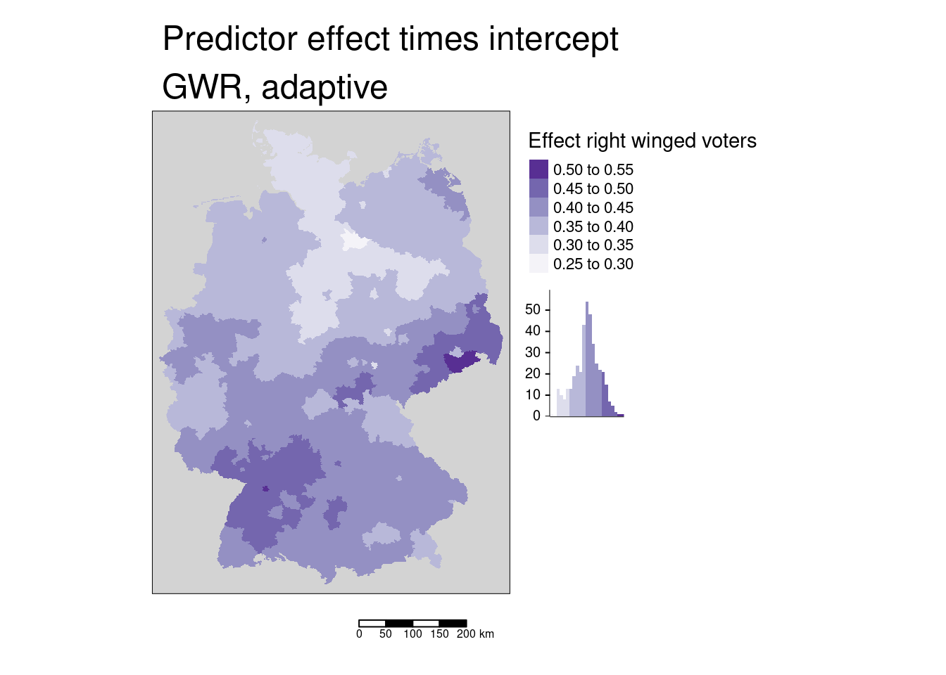
To get the expected cases this would have to be multiplied by the inhabitants.
We continue with the other predictors.
tmap_mode("plot")
m2 <- tm_shape(gGwrAdaptPo_sf) +
  tm_fill(fill="Auslaenderanteil",
          fill.legend= tm_legend(title = "Coef. for share foreigners", reverse=TRUE),
          fill.scale= tm_scale_intervals(values = "brewer.reds", n=7)
          ) +
  tm_layout(legend.outside = TRUE, bg="lightgrey", attr.outside = TRUE)+
  tm_scalebar(position = tm_pos_out()) + tm_title("GWR regression coefficients, adaptive")

mForeign <- tm_shape(covidKreise) +
  tm_fill(fill="Auslaenderanteil",
          fill.legend= tm_legend(title = "Share foreigners", reverse= TRUE),
          fill.scale= tm_scale_intervals(n=7, values = "brewer.blues")
        ) +
  tm_layout(legend.outside = TRUE, bg="lightgrey", attr.outside = TRUE)+
  tm_scalebar(position = tm_pos_out()) + tm_title("INKAR data")

tmap_arrange(m2, mForeign)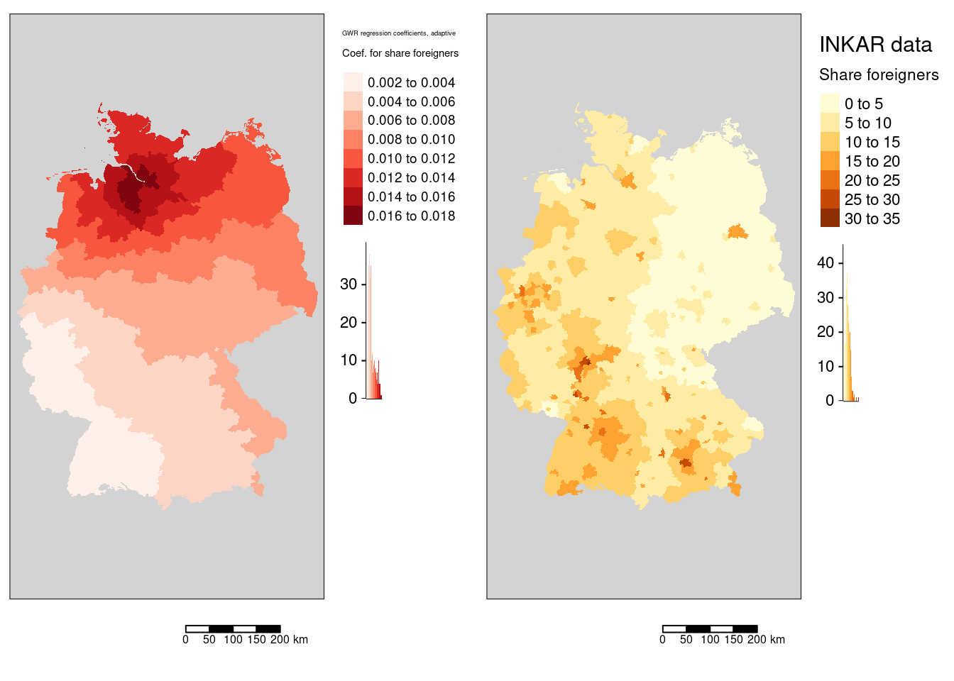
Regression coefficients are always positive. The spatial pattern shows similarities with the share of votes for the AfD GWR coefficient map. The pattern differs in so far, as that the western NRW region is well aligned with the general trend and that for the north-eastern districts the association weakens with increasing distance to Hamburg.
m3 <- tm_shape(gGwrAdaptPo_sf) +
  tm_fill(fill="Hochqualifizierte",
          fill.legend= tm_legend(title="Coef. for highly qualified employees", reverse=TRUE),
          fill.scale = tm_scale_intervals(values = "-brewer.rd_bu")) +
  tm_layout(legend.outside = TRUE, bg="lightgrey", attr.outside = TRUE)+
  tm_scalebar(position = tm_pos_out()) +
  tm_title("GWR regression coefficients, adaptive")

mHighQ <- tm_shape(covidKreise) +
  tm_fill(fill="Hochqualifizierte",
          fill.legend = tm_legend(title = "Share highly qualified employees", reverse = TRUE),
          fill.scale= tm_scale_intervals(values = "brewer.or_rd", n=7)) +
  tm_layout(legend.outside = TRUE, bg="lightgrey", attr.outside = TRUE)+
  tm_scalebar(position = tm_pos_out()) +
  tm_title("INKAR data")

tmap_arrange(m3, mHighQ)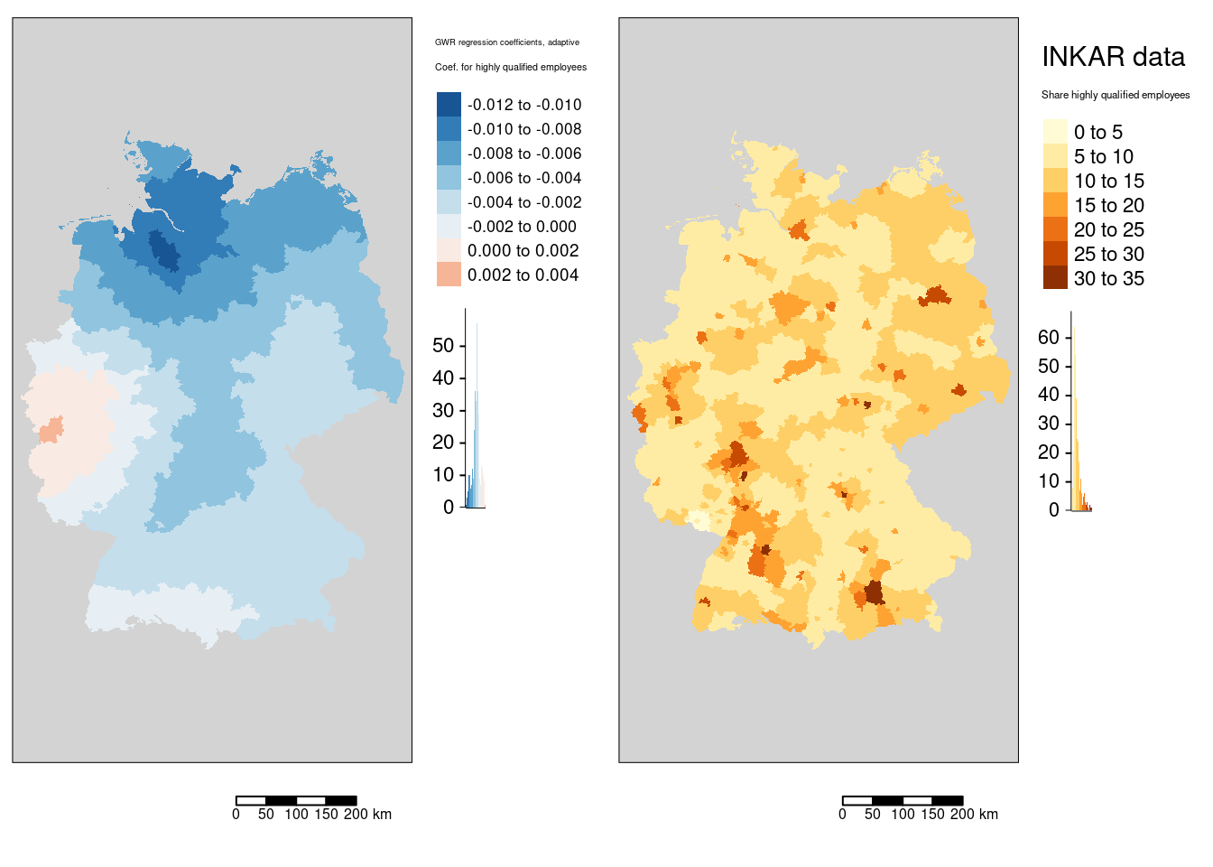
The association between the share of highly qualified employees and the COVID-19 rates is always negative with the exception of the western districts in Rhineland-Palatina and NRW. The strongest positive association was found for the Kreis Euskirchen.
m4 <- tm_shape(gGwrAdaptPo_sf) +
  tm_fill(fill="Langzeitarbeitslosenquote",
          fill.legend= tm_legend(title="Coef. for long term unemployment rate",  reverse=TRUE),
          fill.scale= tm_scale_intervals(values= "brewer.blues"),
           fill.chart = tm_chart_histogram()) +
  tm_layout( legend.outside = TRUE, bg="lightgrey", attr.outside = TRUE) +
  tm_scalebar() + tm_title("GWR regression coefficients, adaptive")

mLunempl <- tm_shape(covidKreise) +
  tm_fill(fill="Langzeitarbeitslosenquote",
          fill.legend= tm_legend(title = "Long term unemployment rate", reverse=TRUE),
          fill.scale= tm_scale_intervals(n=7),
         fill.chart = tm_chart_histogram()) +
  tm_layout( legend.outside = TRUE, bg="lightgrey", attr.outside = TRUE)+
  tm_scalebar() + tm_title("INKAR data")

tmap_arrange(m4, mLunempl)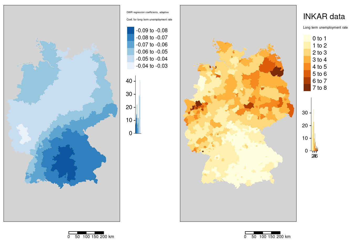
The association between the COVID-19 rate and the long term unemployment rate is always negative. It it strongest in the western part of Bavaria (including Nürnberg, Ulm, Ingolstadt and Augsburg but excluding Munich ) and strong in the rest of Bavaria, southern Saxony and eastern Baden-Württemberg.
m5 <- tm_shape(gGwrAdaptPo_sf) +
  tm_fill(col="Einpendler", title="Coef. for incoming commuters",  legend.hist=TRUE, palette= "Blues") +
  tm_layout(title="GWR regression coefficients, adaptive", legend.outside = TRUE, bg="lightgrey", attr.outside = TRUE)+
  tm_scale_bar()

mIncom <- tm_shape(covidKreise) +
  tm_fill(col="Einpendler", title = "Incoming commuters",
        n=7, legend.hist=TRUE) +
  tm_layout(title="INKAR data", legend.outside = TRUE, bg="lightgrey", attr.outside = TRUE)+
  tm_scale_bar()

tmap_arrange(m5, mIncom)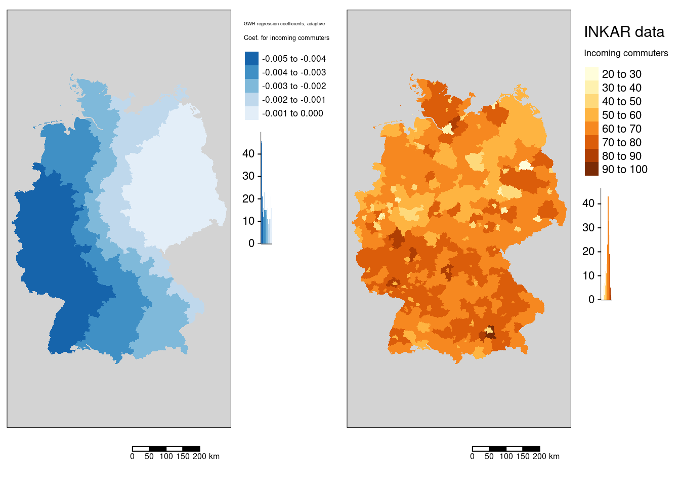
The association of the COVID-19 rate with the incoming commuters is always negative. The spatial pattern is clearly west-east oriented with the highest association in the west of Germany.
m6 <- tm_shape(gGwrAdaptPo_sf) +
  tm_fill(col="Studierende", title="Coef. for share students", palette = "-RdBu", legend.hist=TRUE) +
  tm_layout(title="GWR regression coefficients, adaptive", legend.outside = TRUE, bg="lightgrey", attr.outside = TRUE)+
  tm_scale_bar()

mStudents <- tm_shape(covidKreise) +
  tm_fill(col="Studierende", title = "Share students",
        n=7, legend.hist=TRUE) +
  tm_layout(title="INKAR data", legend.outside = TRUE, bg="lightgrey", attr.outside = TRUE)+
  tm_scale_bar()

tmap_arrange(m6, mStudents)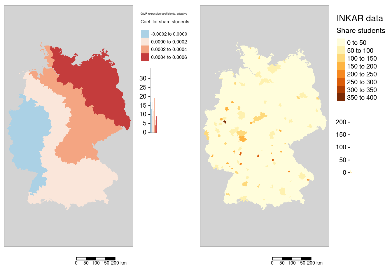
The association between the COVID-19 infection rate and the share of students shows a west to north-east gradient with slightly negative (or non significant?) GWR coefficients in the west.
m7 <- tm_shape(gGwrAdaptPo_sf) +
  tm_fill(col="Laendlichkeit", title="Coef. for rurality", palette = "-RdBu", legend.hist=TRUE) +
  tm_layout(title="GWR regression coefficients, adaptive", legend.outside = TRUE, bg="lightgrey", attr.outside = TRUE)+
  tm_scale_bar()

mRural <- tm_shape(covidKreise) +
  tm_fill(col="Laendlichkeit", title = "Rurality",
        n=7, legend.hist=TRUE) +
  tm_layout(title="INKAR data", legend.outside = TRUE, bg="lightgrey", attr.outside = TRUE)+
  tm_scale_bar()

tmap_arrange(m7, mRural)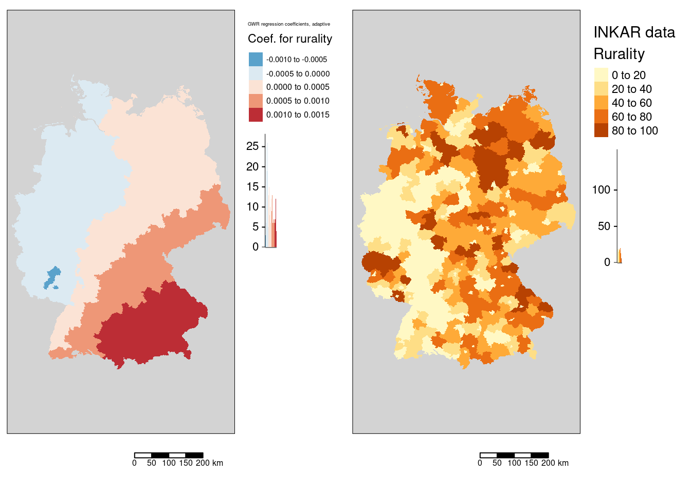
The association between the COVID-19 incidence rate and rurality (the share of the population that lives in places with a low population density) shows a south-east to north-west gradient. Bavaria, parts of Baden-Württemberg, Thüringia and Saxony have a positive association while the western part of Germany shows a negative association. Strongest negative association was found for the districts Bad Kreuznach, Kaiserslautern and Kusel.
How do the residuals look like?
mResid <- tm_shape(gGwrAdaptPo_sf) +
    tm_fill("deviance_resids", title = "Deviance residuals", palette = "-RdBu", n=7) +
    tm_layout(title="Residuals GWR", title.size=.7) +
  tm_layout(title="GWR regression coefficients, adaptive", legend.outside = TRUE, bg="lightgrey", attr.outside = TRUE)+
  tm_scale_bar()
mResid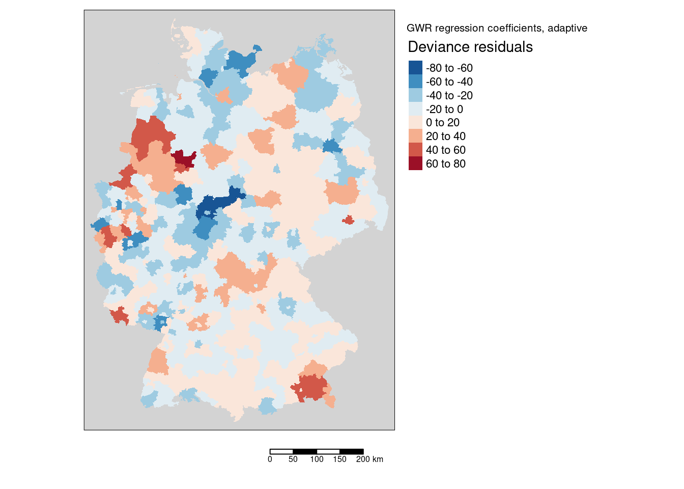
The deviance residuals show no clear overall pattern. Large positive residuals (the model is underestimating the incidence rate) were found in Rosenheim & Traunstein, Saarbrücken, MInden-Lübbeke, Emsland, Cloppenburg, Vechta and Borken.
The following districts showed the largest negative values:
idx <- order(gGwrAdaptPo$SDF$deviance_resids)
#gGwrAdaptPo$SDF$deviance_resids[idx[1:12]]
covidKreiseSp$GEN[idx[1:12]]
## [1] "Kassel" "Göttingen" "Ostholstein"
## [4] "Duisburg" "Steinburg" "Heinsberg"
## [7] "Rhein-Sieg-Kreis" "Südliche Weinstraße" "Plön"
## [10] "Schwalm-Eder-Kreis" "Paderborn" "Berlin"We ordered the data by the size of the residuals (order returns the index and does not sort the data as sort does), then we use the index of the twelfth districts with the smallest (largest negative) residuals to subset the districts names. As the gwr object has the same order as the original (sp or sf) data frame this works fine.
Now let’s combine the plots into one using the mapping capabilities of the tmap package.
We can also plot the fixed bandwidth used based on the adaptive bandwidth, which differs in space. Especially for the districts at the boundary long bandwidths need to be uised to get the required number of neighbors for the local regression.
gGwrAdaptPo_sf$bandwidth <- gGwrAdaptPo$bandwidth

mBW <- tm_shape(gGwrAdaptPo_sf) +
    tm_fill("bandwidth", title = "Bandwidth [m]", palette = "Blues", n=7) +
  tm_layout(title="Realized fixed bandwith, adaptive, optimized", legend.outside = TRUE,
            bg="lightgrey", attr.outside = TRUE)+
  tm_scale_bar()
## ## ── tmap v3 code detected ───────────────────────────────────────────────────────## [v3->v4] `tm_tm_fill()`: migrate the argument(s) related to the scale of the
## visual variable `fill` namely 'n', 'palette' (rename to 'values') to fill.scale
## = tm_scale(<HERE>).
## [v3->v4] `tm_fill()`: migrate the argument(s) related to the legend of the
## visual variable `fill` namely 'title' to 'fill.legend = tm_legend(<HERE>)'
## [v3->v4] `tm_layout()`: use `tm_title()` instead of `tm_layout(title = )`
## ! `tm_scale_bar()` is deprecated. Please use `tm_scalebar()` instead.## [cols4all] color palettes: use palettes from the R package cols4all. Run
## `cols4all::c4a_gui()` to explore them. The old palette name "Blues" is named
## "brewer.blues"
## Multiple palettes called "blues" found: "brewer.blues", "matplotlib.blues". The first one, "brewer.blues", is returned.
##
## [plot mode] fit legend/component: Some legend items or map compoments do not
## fit well, and are therefore rescaled.
## ℹ Set the tmap option `component.autoscale = FALSE` to disable rescaling.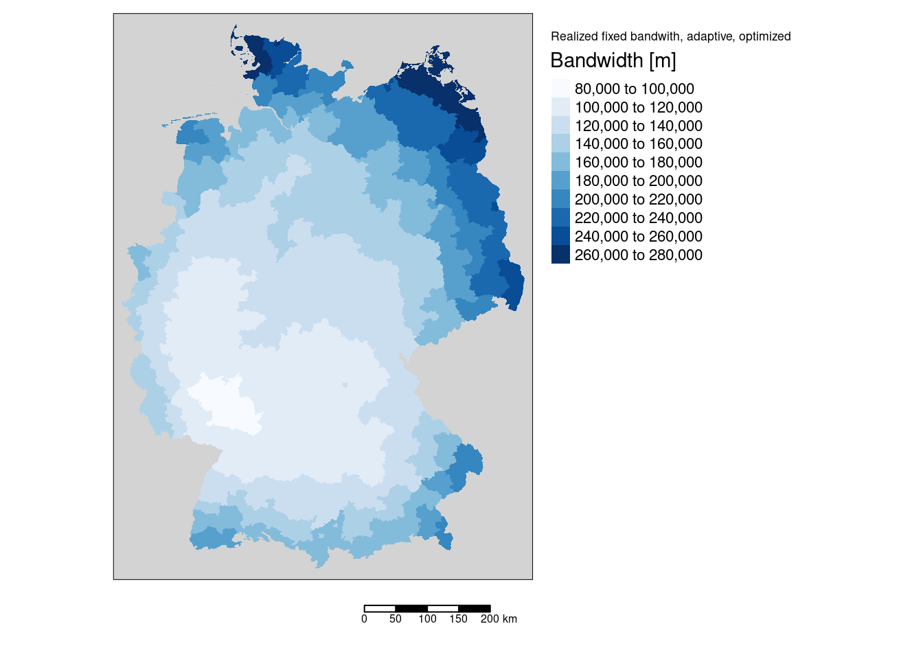
While we always have the same number of neighbors, distances differ, which leads to different weights. This is present in the sum.w column of the SDF slot of the ggwr object and can be plotted as well. We see that the sums of regression weights are not easily predictable as they depend on the realized bandwidth for the location and the distances to the districts
mW <- tm_shape(gGwrAdaptPo_sf) +
    tm_fill("sum.w", title = "Sum of weights", palette = "Blues", n=7) +
  tm_layout(title="GWR regression, adaptive, optimized", legend.outside = TRUE,
            bg="lightgrey", attr.outside = TRUE)+
  tm_scale_bar()
## ## ── tmap v3 code detected ───────────────────────────────────────────────────────## [v3->v4] `tm_tm_fill()`: migrate the argument(s) related to the scale of the
## visual variable `fill` namely 'n', 'palette' (rename to 'values') to fill.scale
## = tm_scale(<HERE>).
## [v3->v4] `tm_fill()`: migrate the argument(s) related to the legend of the
## visual variable `fill` namely 'title' to 'fill.legend = tm_legend(<HERE>)'
## [v3->v4] `tm_layout()`: use `tm_title()` instead of `tm_layout(title = )`
## ! `tm_scale_bar()` is deprecated. Please use `tm_scalebar()` instead.## [cols4all] color palettes: use palettes from the R package cols4all. Run
## `cols4all::c4a_gui()` to explore them. The old palette name "Blues" is named
## "brewer.blues"
## Multiple palettes called "blues" found: "brewer.blues", "matplotlib.blues". The first one, "brewer.blues", is returned.
##
## [plot mode] fit legend/component: Some legend items or map compoments do not
## fit well, and are therefore rescaled.
## ℹ Set the tmap option `component.autoscale = FALSE` to disable rescaling.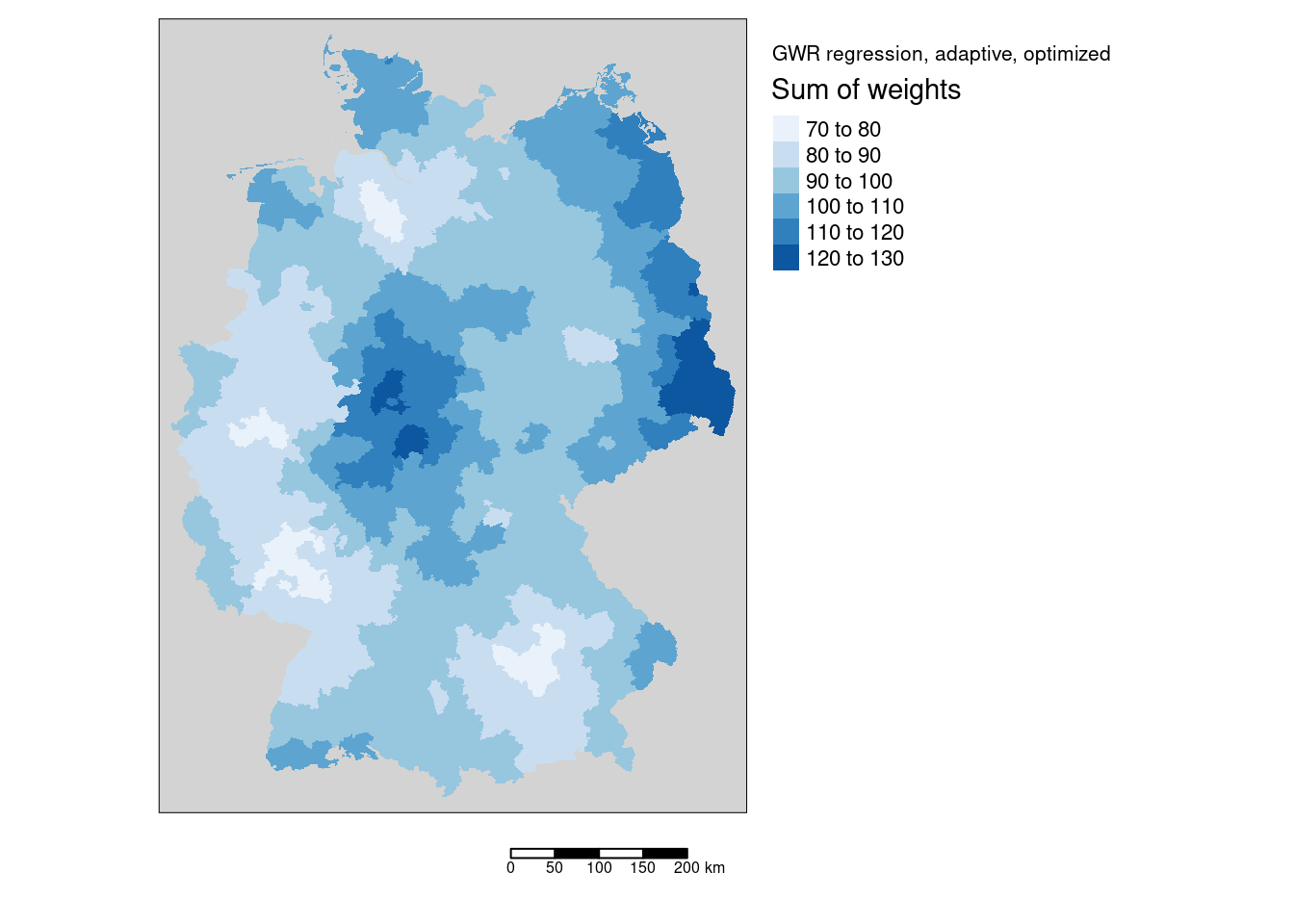
11.3.1.1.1 Collinearity between the GWR coefficients?
As the scatterplot matrix reveals the different coefficients tend to be correlated. This could be caused by a trade-off between the different coefficients.
gGwrAdaptPo$SDF %>% as.data.frame() %>%
  ggpairs(columns = 2:9,
          mapping = aes(alpha=.25), progress = FALSE)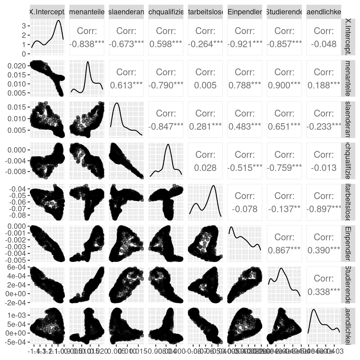
Interestingly, the correlation does not or only partially originate from a correlation in the raw data. The find predictor pairs for which the correlation between GR coefficients is stronger as in the original data (e.g. share of foreigners - share of highly qualified employees) and those were it is weaker (e.g. share foreigners - rurality).
covidKreise %>% st_drop_geometry() %>%
  dplyr::select(c(Stimmenanteile.AfD, Auslaenderanteil, Hochqualifizierte,
           Langzeitarbeitslosenquote, Einpendler, Studierende, Laendlichkeit)) %>%
  cor() %>%
corrplot.mixed(lower= "ellipse", upper = "number", tl.pos = 'lt' )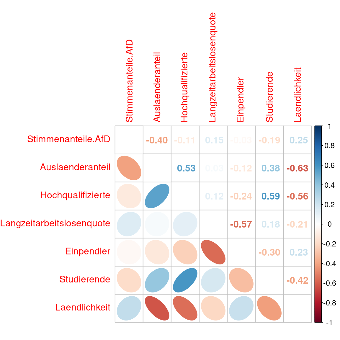
11.3.2 Fixed bandwidth
Instead of using a fixed share of the districts one could as well use a fixed distance for the kernel.
selBandwidth <- ggwr.sel(sumCasesTotal ~ Stimmenanteile.AfD +
                        Auslaenderanteil + Hochqualifizierte +
                        Langzeitarbeitslosenquote + Einpendler  +
                        Studierende + Laendlichkeit + offset(log(EWZ)),
                        adapt = FALSE,family = "poisson", data = covidKreiseSp)
## Bandwidth: 383176.1 CV score: 60699414021
## Bandwidth: 619372.9 CV score: 63184790980
## Bandwidth: 237198.4 CV score: 56738304091
## Bandwidth: 146979.2 CV score: 57765422651
## Bandwidth: 226993.4 CV score: 56441273509
## Bandwidth: 203337.4 CV score: 55944263329
## Bandwidth: 181810.5 CV score: 55975584000
## Bandwidth: 194037.1 CV score: 55879353915
## Bandwidth: 193628.6 CV score: 55878927641
## Bandwidth: 192979.6 CV score: 55878716227
## Bandwidth: 193064 CV score: 55878711081
## Bandwidth: 193066.3 CV score: 55878711078
## Bandwidth: 193066.1 CV score: 55878711078
## Bandwidth: 193066.1 CV score: 55878711078
## Bandwidth: 193066.1 CV score: 55878711078
## Bandwidth: 193065.3 CV score: 55878711079
## Bandwidth: 193065.8 CV score: 55878711078
## Bandwidth: 193065.9 CV score: 55878711078
## Bandwidth: 193066 CV score: 55878711078
## Bandwidth: 193066 CV score: 55878711078
## Bandwidth: 193066 CV score: 55878711078
## Bandwidth: 193066 CV score: 55878711078
## Bandwidth: 193066 CV score: 55878711078
## Bandwidth: 193066 CV score: 55878711078The value suggested by ggwr.sel represents the bandwidth of the kernel (distance in map units) which is meters in our case.
## The selected bandwidth is: 193.1km.gGwrBwPo <- ggwr(sumCasesTotal ~ Stimmenanteile.AfD +
Auslaenderanteil + Hochqualifizierte +
Langzeitarbeitslosenquote + Einpendler +
Studierende + Laendlichkeit + offset(log(EWZ)),
family = "quasipoisson", data = covidKreiseSp, bandwidth = selBandwidth, type="deviance")## Warning in proj4string(data): CRS object has comment, which is lost in output; in tests, see
## https://cran.r-project.org/web/packages/sp/vignettes/CRS_warnings.html## Call:
## ggwr(formula = sumCasesTotal ~ Stimmenanteile.AfD + Auslaenderanteil +
## Hochqualifizierte + Langzeitarbeitslosenquote + Einpendler +
## Studierende + Laendlichkeit + offset(log(EWZ)), data = covidKreiseSp,
## bandwidth = selBandwidth, family = "quasipoisson", type = "deviance")
## Kernel function: gwr.Gauss
## Fixed bandwidth: 193066
## Summary of GWR coefficient estimates at data points:
## Min. 1st Qu. Median 3rd Qu.
## X.Intercept. -1.5108e+00 -1.2550e+00 -1.1480e+00 -1.0784e+00
## Stimmenanteile.AfD 1.0848e-02 1.4219e-02 1.5468e-02 1.7898e-02
## Auslaenderanteil 3.0497e-03 5.5231e-03 6.6069e-03 8.3391e-03
## Hochqualifizierte -1.0803e-02 -4.5401e-03 -3.1863e-03 -2.4218e-03
## Langzeitarbeitslosenquote -7.5882e-02 -6.1469e-02 -5.3150e-02 -4.8549e-02
## Einpendler -4.3506e-03 -3.4723e-03 -2.6812e-03 -1.7767e-03
## Studierende -5.7108e-05 6.5410e-05 1.5834e-04 2.7604e-04
## Laendlichkeit -1.7564e-04 4.7984e-05 3.7099e-04 7.2816e-04
## Max. Global
## X.Intercept. -9.8652e-01 -1.2637
## Stimmenanteile.AfD 2.3031e-02 0.0179
## Auslaenderanteil 1.8439e-02 0.0091
## Hochqualifizierte -6.0122e-04 -0.0045
## Langzeitarbeitslosenquote -4.2566e-02 -0.0557
## Einpendler -1.1017e-04 -0.0016
## Studierende 7.8712e-04 0.0003
## Laendlichkeit 1.3145e-03 0.0005Histogram of local coefficients
globalLmBw <-data.frame(coefficients(gGwrBwPo$lm))
names(globalLmBw) <- "Coefficient.global"
globalLmBw$Predictor <- row.names(globalLmBw)
idx <- which(globalLmBw$Predictor == "(Intercept)")
globalLmBw$Predictor[idx] <- "X.Intercept."
globalLmBw$type <- "Global"


gGwrBwPo$SDF %>% as.data.frame() %>%
  dplyr::select(X.Intercept.:Laendlichkeit) %>%
  pivot_longer(cols = everything(), names_to = "Predictor",
               values_to = "Coefficient") %>%
  ggplot(mapping= aes(x=Coefficient)) + geom_histogram(bins=50) +
  geom_vline(mapping = aes(xintercept = 0, color = "zero"), lty = 2, show.legend=TRUE)  +
  facet_wrap(~ Predictor, scales = "free") +
  geom_vline(aes(xintercept= Coefficient.global, color="global"), data=globalLmBw, lty=2, show.legend=TRUE) +
  scale_color_manual(name = "Reference",
                     values= c(zero = "blue", global = "red"))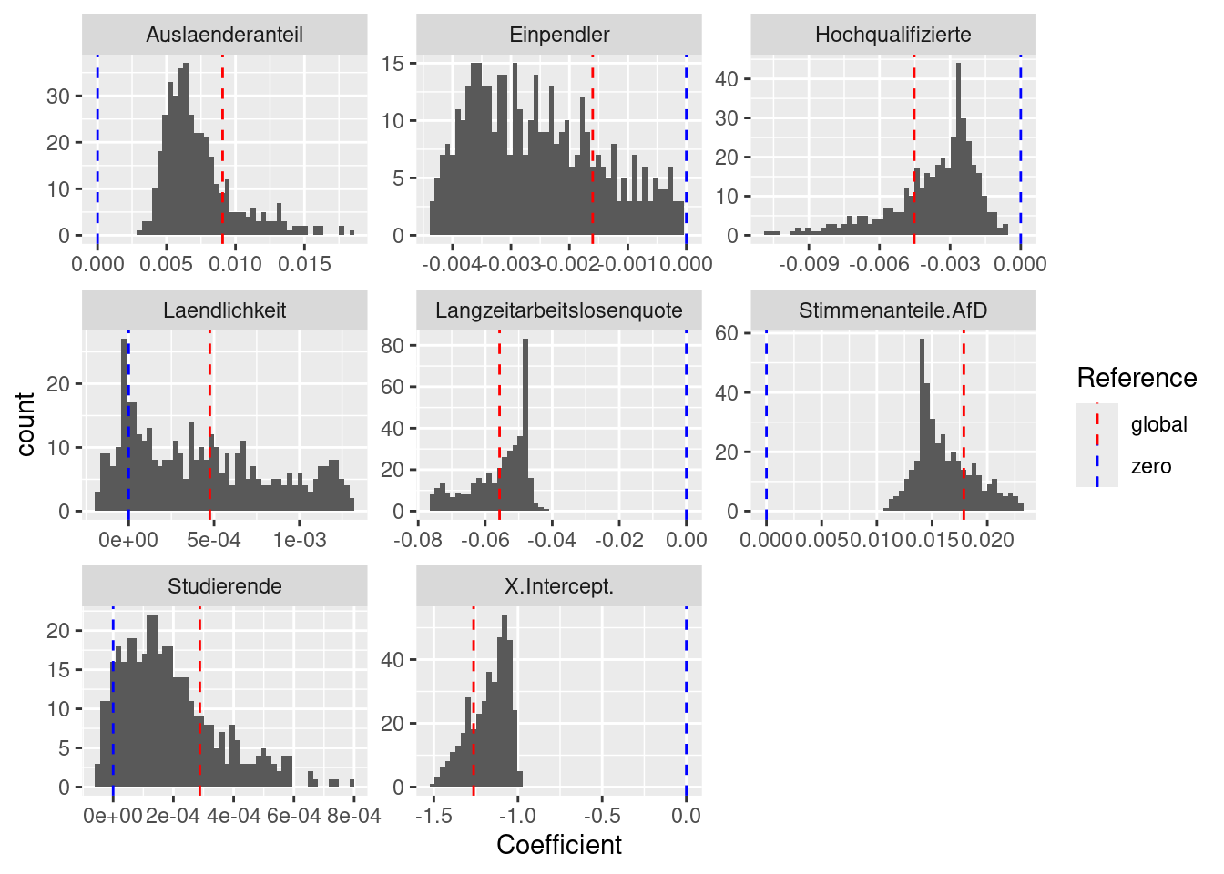
To get an overview about how many data points were used for the regression coefficient at each district, we can use at the sum of the weights. If that distribution is very uneven or if single districts have a sum of weights close to 1 we should become skeptical as this indicates, that the sample size for this districts have been potentially too low for a model of the complexity we are using. The weights result from the kernel used, points far away get less weight, the maximum is one (for the district itself).
##    Min. 1st Qu.  Median    Mean 3rd Qu.    Max.
##   57.67  126.14  157.95  152.33  181.69  212.06
The distribution indicates that we should have for most districts reliable size of data points to estimate a model with seven parameters plus intercept. The distribution is however more widespread compared to the adaptive bandwidth GGWR.
p1 <- ggplot(data= gGwrBwPo$SDF %>% as.data.frame(), aes(x=sum.w)) +
  geom_histogram() +
  xlab("Sum of weights for each district") +
  labs(title = paste("Fixed bandwidth", round(selBandwidth/1000, 1), "km."))

p2 <- ggplot(data= gGwrAdaptPo$SDF %>% as.data.frame(), aes(x=sum.w)) +
  geom_histogram() +
  xlab("Sum of weights for each district") +
  labs(title = paste("Adaptive bandwidth", round(adaptPerc*100,2), "%."))

ggarrange(p1,p2)
## `stat_bin()` using `bins = 30`. Pick better value with `binwidth`.
## `stat_bin()` using `bins = 30`. Pick better value with `binwidth`.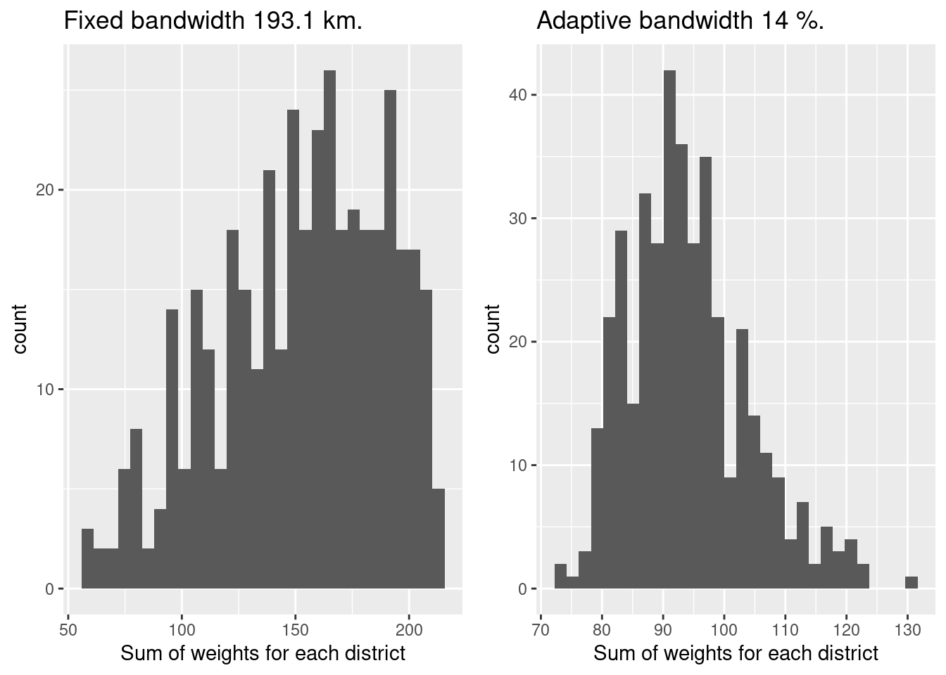
We can also check for the dispersion estimated for the quasi likelihood approach:
## Min. 1st Qu. Median Mean 3rd Qu. Max.
## 69.59 177.99 248.65 237.31 297.44 362.07We see that we have quite some overdispersion in the data - which was expected given the global regression model we have fitted previously.
Convert to sf object:
# creating maps, store them in objects for later display
tmap_mode("plot")
m1bw <- tm_shape(gGwrBwPo_sf) +
tm_fill(col="Stimmenanteile.AfD", title = "Coef. for right winged voters",
palette= "Reds", n=7, legend.hist=TRUE) +
tm_layout(title="GWR regression coefficients, fixed, optimized", legend.outside = TRUE,
bg="lightgrey", attr.outside = TRUE)+
tm_scale_bar()
m2bw <- tm_shape(gGwrBwPo_sf) +
tm_fill(col="Auslaenderanteil", title = "Coef. for share foreigners",
palette= "Reds", n=7, legend.hist=TRUE) +
tm_layout(title="GWR regression coefficients, fixed, optimized", legend.outside = TRUE,
bg="lightgrey", attr.outside = TRUE)+
tm_scale_bar()
m3bw <- tm_shape(gGwrBwPo_sf) +
tm_fill(col="Hochqualifizierte", title="Coef. for highly qualified employees", palette = "Blues", legend.hist=TRUE) +
tm_layout(title="GWR regression coefficients, fixed, optimized", legend.outside = TRUE,
bg="lightgrey", attr.outside = TRUE)+
tm_scale_bar()
m4bw <- tm_shape(gGwrBwPo_sf) +
tm_fill(col="Langzeitarbeitslosenquote", palette = "Blues",
title="Coef. for hlong term unemployment rate", legend.hist=TRUE) +
tm_layout(title="GWR regression coefficients, fixed, optimized", legend.outside = TRUE,
bg="lightgrey", attr.outside = TRUE)+
tm_scale_bar()
m5bw <- tm_shape(gGwrBwPo_sf) +
tm_fill(col="Einpendler", title="Coef. for incoming commuters",
palette= "Blues", legend.hist=TRUE) +
tm_layout(title="GWR regression coefficients, fixed, optimized", legend.outside = TRUE,
bg="lightgrey", attr.outside = TRUE)+
tm_scale_bar()
m6bw <- tm_shape(gGwrBwPo_sf) +
tm_fill(col="Studierende", title="Coef. for share students", palette = "-RdBu", legend.hist=TRUE) +
tm_layout(title="GWR regression coefficients, fixed, optimized", legend.outside = TRUE,
bg="lightgrey", attr.outside = TRUE)+
tm_scale_bar()
m7bw <- tm_shape(gGwrBwPo_sf) +
tm_fill(col="Laendlichkeit", title="Coef. for rurality", palette = "-RdBu", legend.hist=TRUE) +
tm_layout(title="GWR regression coefficients, fixed, optimized", legend.outside = TRUE,
bg="lightgrey", attr.outside = TRUE)+
tm_scale_bar()
mResidbw <- tm_shape(gGwrBwPo_sf) +
tm_fill("deviance_resids", title = "Deviance residuals", palette = "-RdBu", n=7) +
tm_layout(title="Residuals GWR", title.size=.7) +
tm_layout(title="GWR regression coefficients, n fixed, optimized", legend.outside = TRUE,
bg="lightgrey", attr.outside = TRUE)+
tm_scale_bar()
mWbw <- tm_shape(gGwrBwPo_sf) +
tm_fill("sum.w", title = "Sum of weights", palette = "Blues", n=7) +
tm_layout(title="Sum of weights", title.size=.7) +
tm_layout(title="GWR regression coefficients, fixed, optimized", legend.outside = TRUE,
bg="lightgrey", attr.outside = TRUE)+
tm_scale_bar()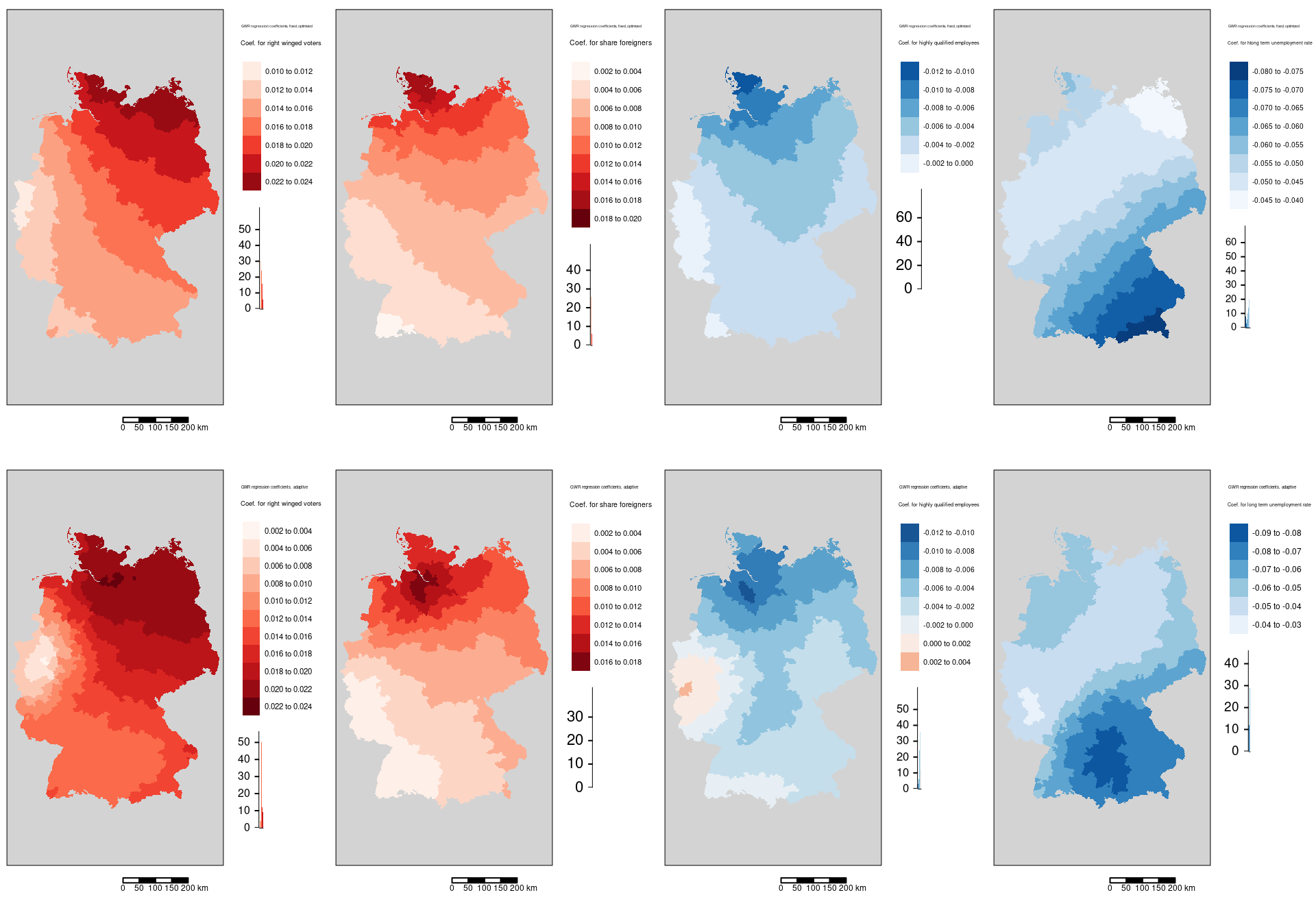
The spatial pattern largely is similar but there are smaller deviations which originate from the different size of the districts. Furthermore, the differences originate from the fact that the adaptive kernel selects the same amount of districts while the non adaptive kernel leads to lower numbers of districts selected for districts at the border of Germany. The first three maps (votes for the AfD, share foreigners and share of highly qualified employees) for the distance bandwidth do not show the strongest association for Hamburg. The association of the incidence rate with the long term unemployment rate does not show a peak in western Bavaria but instead a vewry clear south-east to north-west gradient.
The top row shows the GWR coefficients for the distance bandwidth kernel, the lower one the coefficients for the adaptive kernel.
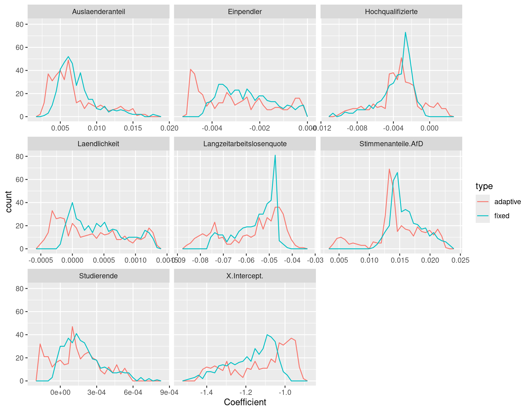
We could also look at the distribution of the coefficients by means of histograms. First, we combine the data from both models in a long format and assign a factor level for each of the two GWR models.
coefFixed <- gGwrBwPo$SDF@data
coefFixed$type <- "fixed"
coefAdapt <- gGwrAdaptPo$SDF@data
coefAdapt$type <- "adaptive"
gwrCoef <- rbind(coefFixed, coefAdapt)
gwrCoef_long <- gwrCoef %>% dplyr::select(c(X.Intercept.:Laendlichkeit, type)) %>%
pivot_longer(cols = X.Intercept.:Laendlichkeit,
names_to = "Predictor", values_to = "Coefficient")
ggplot(gwrCoef_long, mapping = aes(x=Coefficient, colour = type)) +
geom_freqpoly() +
facet_wrap(~Predictor, scales = "free_x")## `stat_bin()` using `bins = 30`. Pick better value with `binwidth`.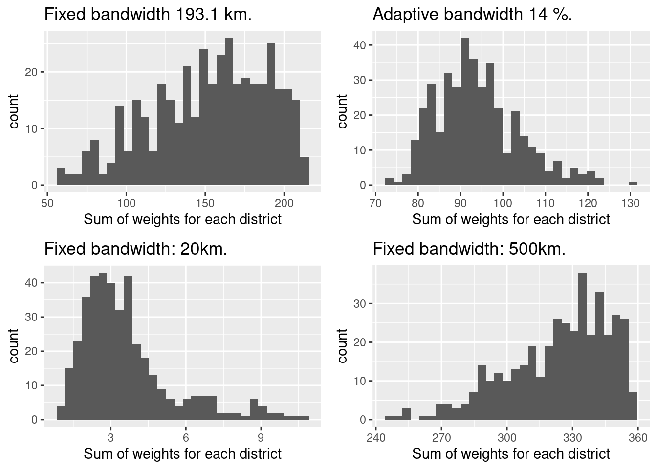
We see that the distribution of the coefficients resembles a similar pattern for both the selected fixed bandwidth and the adaptive kernel size. However, we also can spot differences:
- for long term unemployment rate coefficients show a narrow peak for the fixed bandwidth while for the adaptive kernel we see heavier tails.
- for incomming commuter the adaptive kernel estimated a peak for coefficients between-0.005 and -0.0045 while we had no coefficients in this range for the fixed bandwidth kernel
- for the share of students we see that for the adaptive kernel we had more districts with negative coefficients than for the fixed bandwidth
11.3.3 Testing the effect of different fixed bandwidths
To explore a bit on how the fixed bandwidth influences local coefficients we try two parametes in addition to the optimized bandwidth: 20 and 500km.
20km fixed bandwidth
gGwrBwPo_20 <- ggwr(sumCasesTotal ~ Stimmenanteile.AfD +
Auslaenderanteil + Hochqualifizierte +
Langzeitarbeitslosenquote + Einpendler +
Studierende + Laendlichkeit + offset(log(EWZ)),
family = "quasipoisson", data = covidKreiseSp, bandwidth = 20*10^3, type="deviance")
(gGwrBwPo_20)## Call:
## ggwr(formula = sumCasesTotal ~ Stimmenanteile.AfD + Auslaenderanteil +
## Hochqualifizierte + Langzeitarbeitslosenquote + Einpendler +
## Studierende + Laendlichkeit + offset(log(EWZ)), data = covidKreiseSp,
## bandwidth = 20 * 10^3, family = "quasipoisson", type = "deviance")
## Kernel function: gwr.Gauss
## Fixed bandwidth: 20000
## Summary of GWR coefficient estimates at data points:
## Min. 1st Qu. Median 3rd Qu.
## X.Intercept. -7.30140560 -1.88795670 -1.37988071 -1.02932061
## Stimmenanteile.AfD -0.09027586 -0.00187636 0.01091183 0.02655076
## Auslaenderanteil -0.14021283 -0.00475831 0.00536499 0.01860127
## Hochqualifizierte -0.12715950 -0.00924709 -0.00088571 0.00776872
## Langzeitarbeitslosenquote -0.28861312 -0.05181653 -0.01475801 0.02347795
## Einpendler -0.02519837 -0.00403654 -0.00041863 0.00496734
## Studierende -0.01994965 -0.00087809 -0.00012289 0.00075605
## Laendlichkeit -0.01214971 -0.00078659 0.00056579 0.00187889
## Max. Global
## X.Intercept. 3.30134392 -1.2637
## Stimmenanteile.AfD 0.23610877 0.0179
## Auslaenderanteil 0.29955042 0.0091
## Hochqualifizierte 0.16721840 -0.0045
## Langzeitarbeitslosenquote 0.40398612 -0.0557
## Einpendler 0.04040494 -0.0016
## Studierende 0.01465740 0.0003
## Laendlichkeit 0.01390025 0.0005500km fixed bandwidth
gGwrBwPo_500 <- ggwr(sumCasesTotal ~ Stimmenanteile.AfD +
Auslaenderanteil + Hochqualifizierte +
Langzeitarbeitslosenquote + Einpendler +
Studierende + Laendlichkeit + offset(log(EWZ)),
family = "quasipoisson", data = covidKreiseSp, bandwidth = 500*10^3, type="deviance")
(gGwrBwPo_500)## Call:
## ggwr(formula = sumCasesTotal ~ Stimmenanteile.AfD + Auslaenderanteil +
## Hochqualifizierte + Langzeitarbeitslosenquote + Einpendler +
## Studierende + Laendlichkeit + offset(log(EWZ)), data = covidKreiseSp,
## bandwidth = 500 * 10^3, family = "quasipoisson", type = "deviance")
## Kernel function: gwr.Gauss
## Fixed bandwidth: 5e+05
## Summary of GWR coefficient estimates at data points:
## Min. 1st Qu. Median 3rd Qu.
## X.Intercept. -1.30306354 -1.26603269 -1.24925341 -1.23573933
## Stimmenanteile.AfD 0.01649638 0.01709819 0.01742989 0.01792976
## Auslaenderanteil 0.00766329 0.00824108 0.00853875 0.00904755
## Hochqualifizierte -0.00537791 -0.00468447 -0.00431009 -0.00405779
## Langzeitarbeitslosenquote -0.05896356 -0.05621404 -0.05498551 -0.05372332
## Einpendler -0.00203479 -0.00184548 -0.00169996 -0.00157394
## Studierende 0.00020921 0.00024312 0.00026278 0.00028994
## Laendlichkeit 0.00021841 0.00037610 0.00047565 0.00056071
## Max. Global
## X.Intercept. -1.21026505 -1.2637
## Stimmenanteile.AfD 0.01901443 0.0179
## Auslaenderanteil 0.00994856 0.0091
## Hochqualifizierte -0.00365542 -0.0045
## Langzeitarbeitslosenquote -0.05229114 -0.0557
## Einpendler -0.00127843 -0.0016
## Studierende 0.00035646 0.0003
## Laendlichkeit 0.00073979 0.0005If we check the sum of weights for each district we see that the 20km bandwidth has not been a good choice as we have many districts with only five or less neighbors with a maximum of below 15. THis is way to low for an appropriate estimation of a regression model. As a rule of thumb we need about 10 observations for the estimation of one parameter. As we are estimating parameters for 7 coefficients plus the intercept and the dispersion parameter we should have around 90 observations in the neighborhood for each district. The sum of weights is not exactly the number of observations (as it is weighted by distance) but it provides a rough estimate for the number o9f observations.
p1 <- ggplot(data= gGwrBwPo$SDF %>% as.data.frame(), aes(x=sum.w)) +
geom_histogram() +
xlab("Sum of weights for each district") +
labs(title = paste("Fixed bandwidth", round(selBandwidth/1000, 1), "km."))
p2 <- ggplot(data= gGwrAdaptPo$SDF %>% as.data.frame(), aes(x=sum.w)) +
geom_histogram() +
xlab("Sum of weights for each district") +
labs(title = paste("Adaptive bandwidth", round(adaptPerc*100,2), "%."))
p3 <- ggplot(data= gGwrBwPo_20$SDF %>% as.data.frame(), aes(x=sum.w)) +
geom_histogram() +
xlab("Sum of weights for each district") +
labs(title = "Fixed bandwidth: 20km.")
p4 <- ggplot(data= gGwrBwPo_500$SDF %>% as.data.frame(), aes(x=sum.w)) +
geom_histogram() +
xlab("Sum of weights for each district") +
labs(title = "Fixed bandwidth: 500km.")
ggarrange(p1,p2, p3, p4)## `stat_bin()` using `bins = 30`. Pick better value with `binwidth`.
## `stat_bin()` using `bins = 30`. Pick better value with `binwidth`.
## `stat_bin()` using `bins = 30`. Pick better value with `binwidth`.
## `stat_bin()` using `bins = 30`. Pick better value with `binwidth`.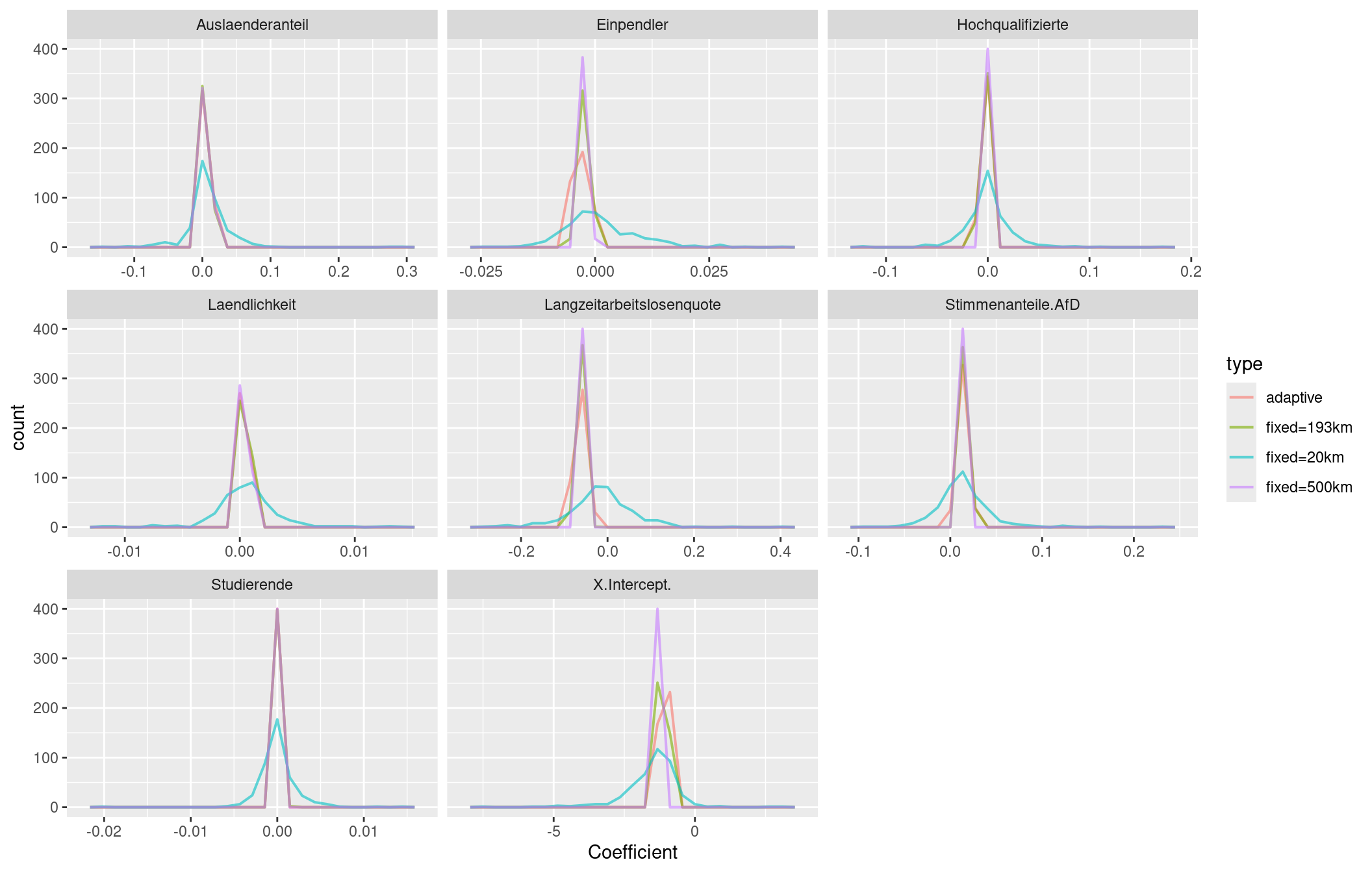
Comparison of the distribution of local regression coefficients
coefFixed <- gGwrBwPo$SDF@data
coefFixed$type <- "fixed=193km"
coefAdapt <- gGwrAdaptPo$SDF@data
coefAdapt$type <- "adaptive"
coefFixed20 <- gGwrBwPo_20$SDF@data
coefFixed20$type <- "fixed=20km"
coefFixed500 <- gGwrBwPo_500$SDF@data
coefFixed500$type <- "fixed=500km"

gwrCoef <- rbind(coefFixed, coefAdapt, coefFixed20, coefFixed500)
gwrCoef_long <- gwrCoef %>% dplyr::select(c(X.Intercept.:Laendlichkeit, type)) %>%
  pivot_longer(cols = X.Intercept.:Laendlichkeit,
             names_to = "Predictor", values_to = "Coefficient")

ggplot(gwrCoef_long, mapping = aes(x=Coefficient, colour = type)) +
  geom_freqpoly(bins = 25, size=.7, alpha=.6) +
  facet_wrap(~Predictor, scales = "free_x")
## Warning: Using `size` aesthetic for lines was deprecated in ggplot2 3.4.0.
## ℹ Please use `linewidth` instead.
## This warning is displayed once every 8 hours.
## Call `lifecycle::last_lifecycle_warnings()` to see where this warning was
## generated.
It is also worth exploring the coefficient maps:
gGwrBwPo_20_sf <- st_as_sf(gGwrBwPo_20$SDF)
gGwrBwPo_500_sf <- st_as_sf(gGwrBwPo_500$SDF)

# creating maps, store them in objects for later display
tmap_mode("plot")
m1bw_20 <- tm_shape(gGwrBwPo_20_sf) +
  tm_fill(col="Stimmenanteile.AfD", title = "Coef. for right winged voters",
          palette= "-RdBu", n=7,
          legend.hist=TRUE, midpoint = 0) +
  tm_layout(title="GWR regression coefficients, 20 km", legend.outside = TRUE, bg="lightgrey", attr.outside = TRUE)+
  tm_scale_bar()

m2bw_20 <- tm_shape(gGwrBwPo_20_sf) +
  tm_fill(col="Auslaenderanteil", title = "Coef. for share foreigners",
          palette= "-RdBu", n=7,
          legend.hist=TRUE, midpoint = 0) +
  tm_layout(title="GWR regression coefficients, 20 km", legend.outside = TRUE, bg="lightgrey", attr.outside = TRUE)+
  tm_scale_bar()

m3bw_20 <- tm_shape(gGwrBwPo_20_sf) +
  tm_fill(col="Hochqualifizierte", title="Coef. for highly qualified employees",
          palette = "-RdBu", legend.hist=TRUE, midpoint = 0) +
  tm_layout(title="GWR regression coefficients, 20 km", legend.outside = TRUE, bg="lightgrey", attr.outside = TRUE)+
  tm_scale_bar()

m4bw_20 <- tm_shape(gGwrBwPo_20_sf) +
  tm_fill(col="Langzeitarbeitslosenquote", palette = "-RdBu",
          title="Coef. for hlong term unemployment rate",
          legend.hist=TRUE, midpoint = 0) +
  tm_layout(title="GWR regression coefficients, 20 km", legend.outside = TRUE, bg="lightgrey", attr.outside = TRUE)+
  tm_scale_bar()

m5bw_20 <- tm_shape(gGwrBwPo_20_sf) +
  tm_fill(col="Einpendler", title="Coef. for incoming commuters",
          palette= "-RdBu", legend.hist=TRUE, midpoint = 0) +
  tm_layout(title="GWR regression coefficients, 20 km", legend.outside = TRUE, bg="lightgrey", attr.outside = TRUE)+
  tm_scale_bar()

m6bw_20 <- tm_shape(gGwrBwPo_20_sf) +
  tm_fill(col="Studierende", title="Coef. for share students",
          palette = "-RdBu", legend.hist=TRUE, midpoint = 0) +
  tm_layout(title="GWR regression coefficients, 20 km", legend.outside = TRUE, bg="lightgrey", attr.outside = TRUE)+
  tm_scale_bar()

m7bw_20 <- tm_shape(gGwrBwPo_20_sf) +
  tm_fill(col="Laendlichkeit", title="Coef. for rurality",
          palette = "-RdBu", legend.hist=TRUE, midpoint = 0) +
  tm_layout(title="GWR regression coefficients, 20 km", legend.outside = TRUE, bg="lightgrey", attr.outside = TRUE)+
  tm_scale_bar()

mResidbw_20 <- tm_shape(gGwrBwPo_20_sf) +
    tm_fill("deviance_resids", title = "Deviance residuals", palette = "-RdBu", n=7) +
    tm_layout(title="Residuals GWR", title.size=.7) +
  tm_layout(title="GWR regression coefficients, 20 km", legend.outside = TRUE, bg="lightgrey", attr.outside = TRUE)+
  tm_scale_bar()

mWbw_20 <- tm_shape(gGwrBwPo_20_sf) +
    tm_fill("sum.w", title = "Sum of weights", palette = "Blues", n=7) +
    tm_layout(title="Sum of weights", title.size=.7) +
  tm_layout(title="GWR regression coefficients, 20 km", legend.outside = TRUE, bg="lightgrey", attr.outside = TRUE)+
tm_scale_bar()tmap_mode("plot")
m1bw_500 <- tm_shape(gGwrBwPo_500_sf) +
tm_fill(col="Stimmenanteile.AfD", title = "Coef. for right winged voters",
palette= "-RdBu", n=7, legend.hist=TRUE, midpoint = 0) +
tm_layout(title="GWR regression coefficients, 500 km", legend.outside = TRUE, bg="lightgrey", attr.outside = TRUE)+
tm_scale_bar()
m2bw_500 <- tm_shape(gGwrBwPo_500$SDF) +
tm_fill(col="Auslaenderanteil", title = "Coef. for share foreigners",
palette= "-RdBu", n=7, legend.hist=TRUE, midpoint = 0) +
tm_layout(title="GWR regression coefficients, 500 km", legend.outside = TRUE, bg="lightgrey", attr.outside = TRUE)+
tm_scale_bar()
m3bw_500 <- tm_shape(gGwrBwPo_500_sf) +
tm_fill(col="Hochqualifizierte", title="Coef. for highly qualified employees",
palette = "-RdBu", legend.hist=TRUE, midpoint = 0) +
tm_layout(title="GWR regression coefficients, 500 km", legend.outside = TRUE, bg="lightgrey", attr.outside = TRUE)+
tm_scale_bar()
m4bw_500 <- tm_shape(gGwrBwPo_500_sf) +
tm_fill(col="Langzeitarbeitslosenquote", palette = "-RdBu",
title="Coef. for hlong term unemployment rate",
legend.hist=TRUE, midpoint = 0) +
tm_layout(title="GWR regression coefficients, 500 km", legend.outside = TRUE, bg="lightgrey", attr.outside = TRUE)+
tm_scale_bar()
m5bw_500 <- tm_shape(gGwrBwPo_500_sf) +
tm_fill(col="Einpendler", title="Coef. for incoming commuters",
palette= "Blues", legend.hist=TRUE, midpoint = 0) +
tm_layout(title="GWR regression coefficients, 500 km", legend.outside = TRUE, bg="lightgrey", attr.outside = TRUE)+
tm_scale_bar()
m6bw_500 <- tm_shape(gGwrBwPo_500_sf) +
tm_fill(col="Studierende", title="Coef. for share students", palette = "-RdBu",
legend.hist=TRUE, midpoint = 0) +
tm_layout(title="GWR regression coefficients, 500 km", legend.outside = TRUE, bg="lightgrey", attr.outside = TRUE)+
tm_scale_bar()
m7bw_500 <- tm_shape(gGwrBwPo_500_sf) +
tm_fill(col="Laendlichkeit", title="Coef. for rurality", palette = "-RdBu",
legend.hist=TRUE, midpoint = 0) +
tm_layout(title="GWR regression coefficients, 500 km", legend.outside = TRUE, bg="lightgrey", attr.outside = TRUE)+
tm_scale_bar()
mResidbw_500 <- tm_shape(gGwrBwPo_500_sf) +
tm_fill("deviance_resids", title = "Deviance residuals", palette = "-RdBu", n=7, midpoint = 0) +
tm_layout(title="Residuals GWR", title.size=.7) +
tm_layout(title="GWR regression coefficients, 500 km", legend.outside = TRUE, bg="lightgrey", attr.outside = TRUE)+
tm_scale_bar()
mWbw_500 <- tm_shape(gGwrBwPo_500_sf) +
tm_fill("sum.w", title = "Sum of weights", palette = "Blues", n=7) +
tm_layout(title="Sum of weights", title.size=.7) +
tm_layout(title="GWR regression coefficients, 500 km", legend.outside = TRUE, bg="lightgrey", attr.outside = TRUE)+
tm_scale_bar()For the share of votes for the right-winged party (AfD) we see that for the 20km distance band much more localized effects. For many rural areas we will have only a few neighbors. Therefore, the coefficients represents artefacts. Presumably many of them are not significantly different from zero, especially if we would correct for multiple testing - e.g. by means of the Holm correction. Please note, that the legend classification differs between the 4 maps and that we even got a change in sign for the 20km bandwidth.
For the 500km bandwidth the north-east to south-west gradient is more linear compared to the optimized bandwidth of 193 km. As we include more neighbors, the surface is generally smoother and local regression coefficients have a reduced range. For 500km bandwidth we miss the Ruhrgebiet as a region of low coefficient values that has been indicated for the 193km and the adaptive kernel.
As a take home message: it is important to pick the bandwidth carefully. Furthermore, as stated above: do not blindly trust the automatic bandwidth selection process but question it from the thematic domain.
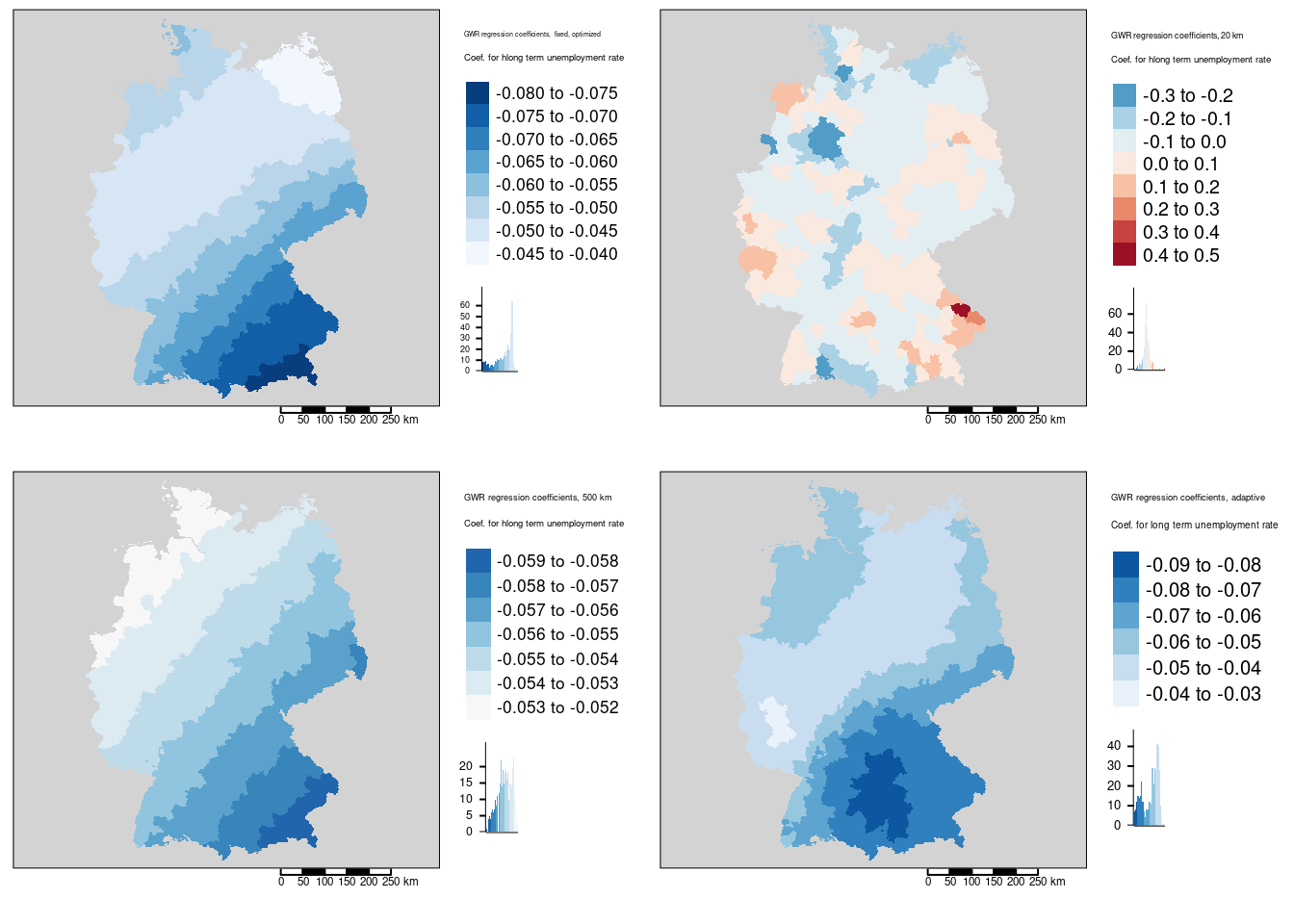
If we compare the local regression coefficients for the four different neighborhood definitions for the long term unemployment rate we detect similar differences. Clearly the 20km bandwidth is to small and leads to artefacts. The larger bandwidth of 500km leads to a relatively smooth north-west to south east gradient for the regression coefficient while the optimized fixed bandwidth of about 193 km presents some more local patterns in the northern part of the country. The adaptive bandwidth identified some local pattern in western Bavaria/eastern Bade-Württemberg and in the Palatinian forest (Pfälzer Wald).
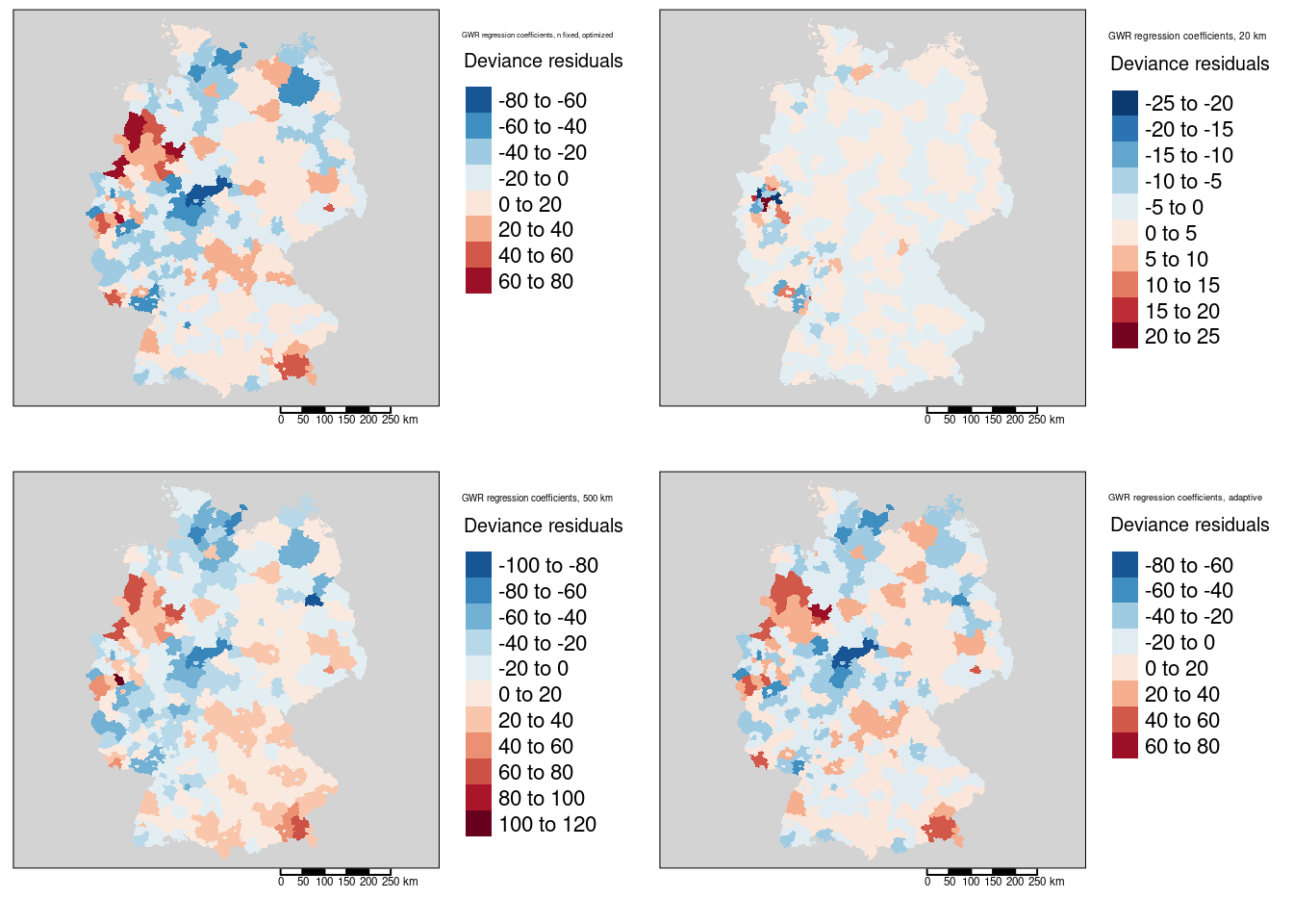
The maps of the local deviance residuals shows much smaller residuals for the small bandwidth (20km) - which is again likely an artefact as the small neighborhoods lead tend to have lower variability.

11.3.4 Comparing different kernels
Let’s have a look at the effect of different kernels. We will pick the adaptive kernel and compare it for the gaussian kernel (used so far) and the bisquared kernel. As we saw above, the gaussian kernel models spatial relationship continuously, while the bisquared kernel models them discontinuously by setting a hard distance threshold above that all weights are assumed zero.
We are using again crossvalidation to find the “optimal” bandwidth for the bisquared kernel. The structural part of the model is unchanged.
adaptPerc_bisq <- ggwr.sel(sumCasesTotal ~ Stimmenanteile.AfD +
                        Auslaenderanteil + Hochqualifizierte +
                        Langzeitarbeitslosenquote + Einpendler  +
                        Studierende + Laendlichkeit + offset(log(EWZ)),
                        adapt = TRUE,family = "quasipoisson", data = covidKreiseSp,
                      gweight= gwr.bisquare)
## Adaptive q: 0.381966 CV score: 59655212871
## Adaptive q: 0.618034 CV score: 61020035955
## Adaptive q: 0.236068 CV score: 40007960878
## Adaptive q: 0.145898 CV score: 49806423731
## Adaptive q: 0.2436946 CV score: 42822647725
## Adaptive q: 0.2021057 CV score: 38389520124
## Adaptive q: 0.1806363 CV score: 43052334655
## Adaptive q: 0.2160037 CV score: 37457271641
## Adaptive q: 0.21492 CV score: 37436521899
## Adaptive q: 0.2140391 CV score: 37454339475
## Adaptive q: 0.2149842 CV score: 37435399546
## Adaptive q: 0.2153736 CV score: 37443267996
## Adaptive q: 0.2150573 CV score: 37436366253
## Adaptive q: 0.2149842 CV score: 37435399546## Selected adaptive bandwidth (% observations): 21.5%.The bandwidth select differs. Before we had a bandwidth (gaussian kernel) of 14 %.`
gGwrAdaptPo_bisq<- ggwr(sumCasesTotal ~ Stimmenanteile.AfD +
                        Auslaenderanteil + Hochqualifizierte +
                        Langzeitarbeitslosenquote + Einpendler  +
                        Studierende + Laendlichkeit + offset(log(EWZ)),
                    family = "quasipoisson", data = covidKreiseSp, adapt=adaptPerc, type="deviance",
                      gweight= gwr.bisquare)
print(gGwrAdaptPo_bisq)
## Call:
## ggwr(formula = sumCasesTotal ~ Stimmenanteile.AfD + Auslaenderanteil +
## Hochqualifizierte + Langzeitarbeitslosenquote + Einpendler +
## Studierende + Laendlichkeit + offset(log(EWZ)), data = covidKreiseSp,
## gweight = gwr.bisquare, adapt = adaptPerc, family = "quasipoisson",
## type = "deviance")
## Kernel function: gwr.bisquare
## Adaptive quantile: 0.1399629 (about 55 of 400 data points)
## Summary of GWR coefficient estimates at data points:
## Min. 1st Qu. Median 3rd Qu.
## X.Intercept. -2.2408e+00 -1.4859e+00 -1.2391e+00 -1.0480e+00
## Stimmenanteile.AfD -1.5853e-02 3.5134e-03 1.1878e-02 1.9153e-02
## Auslaenderanteil -1.5041e-02 2.1791e-03 6.1194e-03 1.0004e-02
## Hochqualifizierte -3.5705e-02 -5.7786e-03 -1.7711e-03 3.0239e-03
## Langzeitarbeitslosenquote -1.0366e-01 -5.5175e-02 -3.3744e-02 -8.6968e-03
## Einpendler -7.8641e-03 -3.5493e-03 -1.6178e-03 -3.7797e-05
## Studierende -2.3119e-03 -2.6880e-04 -9.0369e-05 3.2097e-04
## Laendlichkeit -3.0780e-03 -4.2923e-04 4.9618e-04 1.1761e-03
## Max. Global
## X.Intercept. -5.7967e-01 -1.2637
## Stimmenanteile.AfD 5.4452e-02 0.0179
## Auslaenderanteil 4.0040e-02 0.0091
## Hochqualifizierte 1.9031e-02 -0.0045
## Langzeitarbeitslosenquote 5.9793e-02 -0.0557
## Einpendler 1.1845e-02 -0.0016
## Studierende 3.4049e-03 0.0003
## Laendlichkeit 2.7168e-03 0.0005A comparison of local coefficients for both ggwr models shows clear differences (c.f. figure 11.2): The gaussian kernel shows a much peakier distribution for the local coefficient estimates than the bisquared kernel.
coefAdapt <- gGwrAdaptPo$SDF@data
coefAdapt$type <- "adaptive, gaussian"
coefAdapt_bisq <- gGwrAdaptPo_bisq$SDF@data
coefAdapt_bisq$type <- "adaptive, bisquare"


gwrCoef <- rbind(coefAdapt, coefAdapt_bisq)
gwrCoef_long <- gwrCoef %>% dplyr::select(c(X.Intercept.:Laendlichkeit, type)) %>%
  pivot_longer(cols = X.Intercept.:Laendlichkeit,
             names_to = "Predictor", values_to = "Coefficient")

ggplot(gwrCoef_long, mapping = aes(x=Coefficient, colour = type)) +
  geom_freqpoly(bins = 25, size=.7, alpha=.6) +
  facet_wrap(~Predictor, scales = "free_x")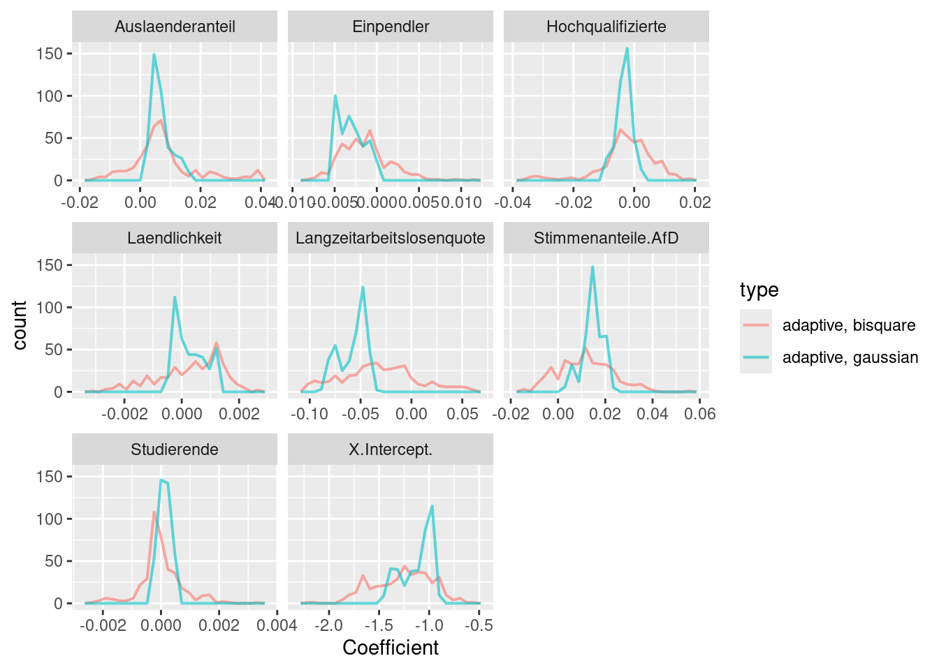
Figure 11.2: Local regression coefficients for the COVID-19 incidence rate ggwr model. Two different kernels (bisquared and gaussian) have been used. For both kernels an adaptive bandwith approach has been used. The adaptive bandwidth (k-nearest neighbors) has been selected - based on CV - for each kernel separately.
The local coefficient maps (figure 11.3 and 11.4) also show clear differences which are caused by the different representation of spatial relationships by the two kernels. The bisquared kernel leads to more local patterns while the gaussian kernel tends to indicate smoother more global patterns.
# creating maps, store them in objects for later display
tmap_mode("plot")
m1_adapt_bisq <- tm_shape(gGwrAdaptPo_bisq_sf) +
  tm_fill(col="Stimmenanteile.AfD", title = "Coef. for right winged voters",
          palette= "-RdBu", n=7, legend.hist=TRUE) +
  tm_layout(title="GWR regression coefficients, adaptive bisquare", legend.outside = TRUE, bg="lightgrey", attr.outside = TRUE)+
  tm_scale_bar()

m2_adapt_bisq <- tm_shape(gGwrAdaptPo_bisq_sf) +
  tm_fill(col="Auslaenderanteil", title = "Coef. for share foreigners",
          palette= "-RdBu", n=7, legend.hist=TRUE) +
  tm_layout(title="GWR regression coefficients, adaptive bisquare", legend.outside = TRUE, bg="lightgrey", attr.outside = TRUE)+
  tm_scale_bar()

m3_adapt_bisq <- tm_shape(gGwrAdaptPo_bisq_sf) +
  tm_fill(col="Hochqualifizierte", title="Coef. for highly qualified employees", palette = "Blues", legend.hist=TRUE) +
  tm_layout(title="GWR regression coefficients, adaptive bisquare", legend.outside = TRUE, bg="lightgrey", attr.outside = TRUE)+
  tm_scale_bar()

m4_adapt_bisq <- tm_shape(gGwrAdaptPo_bisq_sf) +
  tm_fill(col="Langzeitarbeitslosenquote", palette = "-RdBu",
          title="Coef. for hlong term unemployment rate",  legend.hist=TRUE) +
  tm_layout(title="GWR regression coefficients, adaptive bisquare", legend.outside = TRUE, bg="lightgrey", attr.outside = TRUE)+
  tm_scale_bar()

m5_adapt_bisq <- tm_shape(gGwrAdaptPo_bisq_sf) +
  tm_fill(col="Einpendler", title="Coef. for incoming commuters",
          palette= "-RdBu", legend.hist=TRUE) +
  tm_layout(title="GWR regression coefficients, adaptive bisquare", legend.outside = TRUE, bg="lightgrey", attr.outside = TRUE)+
  tm_scale_bar()

m6_adapt_bisq <- tm_shape(gGwrAdaptPo_bisq_sf) +
  tm_fill(col="Studierende", title="Coef. for share students", palette = "-RdBu", legend.hist=TRUE) +
  tm_layout(title="GWR regression coefficients, adaptive bisquare", legend.outside = TRUE, bg="lightgrey", attr.outside = TRUE)+
  tm_scale_bar()

m7_adapt_bisq <- tm_shape(gGwrAdaptPo_bisq_sf) +
  tm_fill(col="Laendlichkeit", title="Coef. for rurality", palette = "-RdBu", legend.hist=TRUE) +
  tm_layout(title="GWR regression coefficients, adaptive bisquare", legend.outside = TRUE, bg="lightgrey", attr.outside = TRUE)+
  tm_scale_bar()

mResid_adapt_bisq <- tm_shape(gGwrAdaptPo_bisq_sf) +
    tm_fill("deviance_resids", title = "Deviance residuals", palette = "-RdBu", n=7) +
    tm_layout(title="Residuals GWR", title.size=.7) +
  tm_layout(title="GWR regression coefficients, adaptive bisquare", legend.outside = TRUE, bg="lightgrey", attr.outside = TRUE)+
  tm_scale_bar()

mW_adapt_bisq <- tm_shape(gGwrAdaptPo_bisq_sf) +
    tm_fill("sum.w", title = "Sum of weights", palette = "Blues", n=7) +
    tm_layout(title="Sum of weights", title.size=.7) +
  tm_layout(title="GWR regression coefficients,  adaptive bisquare", legend.outside = TRUE, bg="lightgrey", attr.outside = TRUE)+
  tm_scale_bar()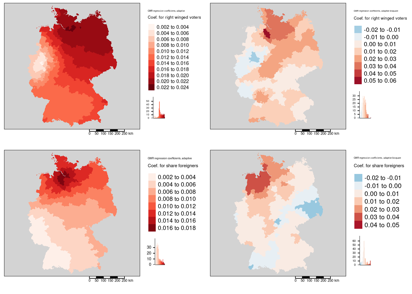
Figure 11.3: Local regression coefficients for the COVID-19 incidence rate ggwr model. Two different kernels (bisquared and gaussian) have been used. For both kernels an adaptive bandwith approach has been used. The adaptive bandwidth (k-nearest neighbors) has been selected - based on CV - for each kernel separately. Coefficients for two predictors are shown: the share of votes for the right-winged parts AfD (top row) and the share of foreigners (bottom row). The gaussian kernel based maps are shown in the first columns, the bisquared kernel based maps in the second column.
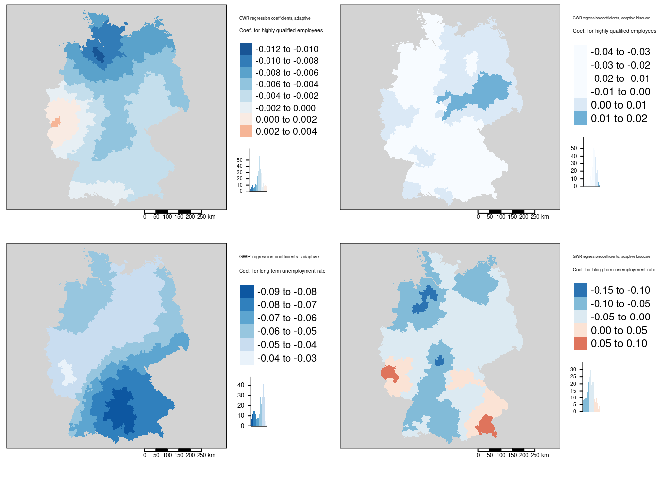
Figure 11.4: Local regression coefficients for the COVID-19 incidence rate ggwr model. Two different kernels (bisquared and gaussian) have been used. For both kernels an adaptive bandwith approach has been used. The adaptive bandwidth (k-nearest neighbors) has been selected - based on CV - for each kernel separately. Coefficients for two predictors are shown: the share of highly qualified employees (top row) and the longterm unemployment rate (bottom row). The gaussian kernel based maps are shown in the first columns, the bisquared kernel based maps in the second column.
The realized fixed bandwidths are exactly the same for both kernel functions after the optimization:
##   [1] 0 0 0 0 0 0 0 0 0 0 0 0 0 0 0 0 0 0 0 0 0 0 0 0 0 0 0 0 0 0 0 0 0 0 0 0 0
##  [38] 0 0 0 0 0 0 0 0 0 0 0 0 0 0 0 0 0 0 0 0 0 0 0 0 0 0 0 0 0 0 0 0 0 0 0 0 0
##  [75] 0 0 0 0 0 0 0 0 0 0 0 0 0 0 0 0 0 0 0 0 0 0 0 0 0 0 0 0 0 0 0 0 0 0 0 0 0
## [112] 0 0 0 0 0 0 0 0 0 0 0 0 0 0 0 0 0 0 0 0 0 0 0 0 0 0 0 0 0 0 0 0 0 0 0 0 0
## [149] 0 0 0 0 0 0 0 0 0 0 0 0 0 0 0 0 0 0 0 0 0 0 0 0 0 0 0 0 0 0 0 0 0 0 0 0 0
## [186] 0 0 0 0 0 0 0 0 0 0 0 0 0 0 0 0 0 0 0 0 0 0 0 0 0 0 0 0 0 0 0 0 0 0 0 0 0
## [223] 0 0 0 0 0 0 0 0 0 0 0 0 0 0 0 0 0 0 0 0 0 0 0 0 0 0 0 0 0 0 0 0 0 0 0 0 0
## [260] 0 0 0 0 0 0 0 0 0 0 0 0 0 0 0 0 0 0 0 0 0 0 0 0 0 0 0 0 0 0 0 0 0 0 0 0 0
## [297] 0 0 0 0 0 0 0 0 0 0 0 0 0 0 0 0 0 0 0 0 0 0 0 0 0 0 0 0 0 0 0 0 0 0 0 0 0
## [334] 0 0 0 0 0 0 0 0 0 0 0 0 0 0 0 0 0 0 0 0 0 0 0 0 0 0 0 0 0 0 0 0 0 0 0 0 0
## [371] 0 0 0 0 0 0 0 0 0 0 0 0 0 0 0 0 0 0 0 0 0 0 0 0 0 0 0 0 0 0
This is also indicated by (but less easy to spot) the maps of the effective bandwidth for both kernels (c.f. figure 11.5)
gGwrAdaptPo_bisq_sf$bandwidth <- gGwrAdaptPo_bisq$bandwidth

mBW_bisq <- tm_shape(gGwrAdaptPo_bisq_sf) +
    tm_fill("bandwidth", title = "Bandwidth [m]", palette = "Blues", n=7) +
  tm_layout(title="Realized fixed bandwith, adaptive, optimized, bisquared", legend.outside = TRUE,
            bg="lightgrey", attr.outside = TRUE)+
  tm_scale_bar()

tmap_arrange(mBW, mBW_bisq)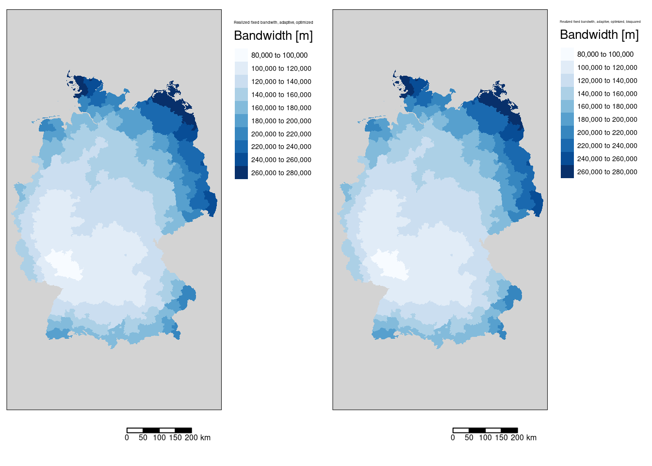
Figure 11.5: Effective bandwidth for the COVID-19 incidence rate ggwr model. Two different kernels (bisquared and gaussian) have been used. For both kernels an adaptive bandwith approach has been used. The adaptive bandwidth (k-nearest neighbors) has been selected - based on CV - for each kernel separately. The gaussian kernel based map is shown in the first columns, the bisquared kernel based map in the second column.
# remove bandwidth to avoid problems with plots when cbinding different SDF objects
#gGwrAdaptPo_bisq$SDF$bandwidth <- NULL
However, the sum of weights differs quite a bit as the bisquared kernel excludes every observation farer away than the bandwidth (c.f. figure 11.6).
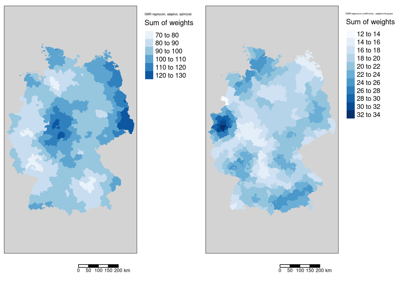
Figure 11.6: Sum of weights for the COVID-19 incidence rate ggwr model. Two different kernels (bisquared and gaussian) have been used. For both kernels an adaptive bandwith approach has been used. The adaptive bandwidth (k-nearest neighbors) has been selected - based on CV - for each kernel separately. The gaussian kernel based map is shown in the first columns, the bisquared kernel based map in the second column.