Chapter 9 Spatial explorative data analysis - local patterns of spatial auto-correlation
So far we have looked at global spatial autocorrelation. A data set might show spatial clustering or show a regular pattern. However, it might be that different parts of the area of interest show different behavior. A part of the data might be clustered while the rest is not showing any spatial pattern. In sum this might lead to a low positive spatial autocorrelation which we might not consider to interesting. However, this spatial pattern in a part of the area of interest might be highly informative as it might indicate for example a missing covariate. It is therefore worth, exploring local patterns as well. In other words, we are now exploring instationarity in the data as well.
## Loading required package: sf## Linking to GEOS 3.12.1, GDAL 3.8.4, PROJ 9.4.0; sf_use_s2() is TRUE## Loading required package: spdep## Loading required package: spData## To access larger datasets in this package, install the spDataLarge
## package with: `install.packages('spDataLarge',
## repos='https://nowosad.github.io/drat/', type='source')`## Loading required package: ncf## Loading required package: tmap## Loading required package: ggplot2## Loading required package: ggpubr## Loading required package: gstat## Loading required package: dplyr##
## Attaching package: 'dplyr'## The following objects are masked from 'package:stats':
##
## filter, lag## The following objects are masked from 'package:base':
##
## intersect, setdiff, setequal, union9.1 Cheat cheet
Required packages:
spdeptmapsf
Important commands:
spdep::localmoran- calculates local Moran’s Ispdep::LOSH- calculate LOSHspdep::localC- calculate local Geary’s Cspdep::localG- calculate local Getis G and Gstarspdep::include.self- include observation \(i\) in the neighborhood (for Getis G)spdep::p.adjustSP- adjust local association measures’ p-valuesstats::p.adjust- “normal” approach to adjust p-values for multiple testing
9.2 Theory
9.2.1 Local Moran’s I
Local Moran’s I (also named LISA) calculates Moran’s I in a neighborhood, check’s significance and compares on the Moran’s I value with the values in the neighborhood (Anselin, 1995).
\[ I_i = \frac{(x_i-\bar{x})}{{∑_{k=1}^{n}(x_k-\bar{x})^2}/(n-1)}{∑_{j=1}^{n}w_{ij}(x_j-\bar{x})} \] With \(i\) the observation (district) index \(w_{ij}\) the element of the spatial weight matrix \(W\), \(x\) the value of interest (here the empirical bayes index of the incidence rate) and \(k\) the number of neighbors of district \(i\).\(\bar{x}\) is the global average.
Local Moran’s I values do not indicate the direction of change: - High values at location i, surrounded by high values in neighborhood -> positive value - Low values at location i, surrounded by low values in neighborhood -> positive value - High values at location i, surrounded by low values in neighborhood -> negative value - Low values at location i, surrounded by high values in neighborhood -> negative value
For the interpretation, local Moran’s I values are categorized (if significant) in comparison to the global mean as well. The following categories (quadrants) are used:
- High – high – value higher than the global mean, surrounded by similar values (cluster of high values)
- Low – low – value lower than the global mean, surrounded by similar values (cluster of low values)
- High –low – high value (compared to the mean) surrounded by dissimilar values (negative spatial autocorrelation), i.e. high local outlier
- Low - high – value lower than the global mean, surrounded by dissimilar values (negative spatial autocorrelation) , i.e. low local outlier
The first part of the quadrant description relates to the value of location \(i\) and the second one to the lagged value. It relates to the four quadrants of the Moran scatterplot.
## Warning in geom_text(aes(2.5, 2.5, label = "High - High")): All aesthetics have length 1, but the data has 2 rows.
## ℹ Please consider using `annotate()` or provide this layer with data containing
##   a single row.
## Warning in geom_text(aes(-2.5, -2.5, label = "Low - Low")): All aesthetics have length 1, but the data has 2 rows.
## ℹ Please consider using `annotate()` or provide this layer with data containing
## a single row.## Warning in geom_text(aes(2.5, -2.5, label = "High - Low")): All aesthetics have length 1, but the data has 2 rows.
## ℹ Please consider using `annotate()` or provide this layer with data containing
## a single row.## Warning in geom_text(aes(-2.5, 2.5, label = "Low - High")): All aesthetics have length 1, but the data has 2 rows.
## ℹ Please consider using `annotate()` or provide this layer with data containing
## a single row.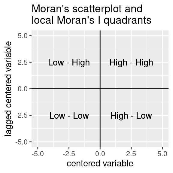
Instead of using the mean to classify the spatial objects with respect to their context, one can as well use the median. Another option (named pysal as this is the default in the python package pysal by Luc Anselin and friends) uses the centered variable and the lagged centred variable splitted at zero as a criterium to classify into the 4 quadrants.
Local Moran’s I is calculated by spdep::localmoran and spdep::localmoran_perm.
The sum of all local Moran’s I values divided by the number of spatial units equals the global Moran’s I.
9.2.2 Adjustmen for multiple testing
The local Moran’s I values can be checked for significance by means of a normal approximation or by a permutation test. As each district is tested separately we run into the problem of multiple testing. In simple words the problem can be described as follows: if we test a lot, some units will be significant just by chance (increased type I error rate, we might fail not reject \(H_0\)). To address this problem several adjustment factors exist which correct the p-vales at the cost of increased type II error rate (we might wrongly reject \(H_0\)). The most conservative and not recommended approach is the bonferoni correction. A suitable alternative that is frequently used is the Holm correction. See ?p.adjust for the other correction methods implemented in R.
For Bonferoni the p-values are multiplied by the number of comparisons. The Holm correction is similar to the Bonferoni approach, but the correction factor only considers hypothesis for observations that are not clearly non-significant (Holm, 1979). There seems no reason to use the unmodified Bonferroni correction because it is dominated by Holm’s method, which is also valid under arbitrary assumptions.
Hochberg’s ("hochberg") and Hommel’s ("hommel") methods are valid when the hypothesis tests are independent or when they are non-negatively associated. Hommel’s method is more powerful than Hochberg’s, but the difference is usually small and the Hochberg p-values are faster to compute. For the case of local measures of association - as considered here - the hypothesis are not independent. Therefore, the two correction methods cannot be used in this context.
The "BH" and "BY" methods of Benjamini, Hochberg, and Yekutieli control the false discovery rate, the expected proportion of false discoveries amongst the rejected hypotheses. The false discovery rate is a less stringent condition than the family-wise error rate, so these methods are more powerful than the others.
We use here the method spdep::p.adjustSP which considers only the number of neighbors of spatial unit \(i\) for the correction, not the total number of spatial units.
9.2.3 Local Geary’s C
Similar to local Moran’s I there exist a local version of Geary’s C. It is calculated as
\[ C_i = \sum_j^n w_{ij}(x_i-x_j)^2 \] It is calculated by spdep::localC and spdep::localC_perm.
Different than for Moran’s I, local Geary’s C do not sum up to the global value. The following proportion factor has to be applied (Anselin, 1995):
\[\gamma = 2n \frac{S_0}{n-1}\]
with \(S_0\) the sum of all weights: \(S_0 = \sum_i\sum_j{w_{i,j}}\)
The factor simplifies for a row standardized spatial weight matrix to:
\[2 \frac{n^2}{n-1}\]
as \(S_0 = n\)
Interpretation of the local Geary’s C values is similar as for local Moran’s I values
9.2.4 Getis G and Gstar
Getis G and Gstar measure how the local mean value compares to the global mean value. The sign indicates the presence of local clusters of high (high value for G or Gstar) or low values (low values for G or Gstar). This makes it easier to interpret than local Moran’s I.
The difference between G and Gstar is the exclusion or the inclusion of the actual spatial unit i in the calcualtaion.
\[ G_i = \frac{\sum_{j, j\neq i}^n w_{ij}x_j}{\sum_{j, j\neq i}^n x_j}\]
\[ G_i^* = \frac{\sum_{j}^n w_{ij}x_j}{\sum_{j}^n x_j}\]
Both values are calculated in R by spdep::localG, the difference between G nd G* is expressed by using a different neighborhood. The command to include the observation \(i\) itself in the neighborhood is spdep::include.self.
For Getis-Ord G* local values are not related to the global statistic.
9.2.5 LOSH - local spatial heteoscedasticity
LOSH measures spatial heterogeneity, how much values differ in the neighborhood. While Getis G looks at the mean value the focus lies here on variability. LOSH is calculated as follows (Ord and Getis, 2012):
\[H_i = \frac{\sum_j^n w_{ij}|e_j|^a}{h_1\sum_j^n w_{ij}} \] with (residual about the local spatially weighted mean)
\[ e_j = x_j - \bar{x}_j\] and (local spatially weighted mean)
\[ \bar{x}_j = \frac{\sum_k^n w_{jk}x_k}{\sum_k^n w_{jk}} \]
and
\[ h_1 = \sum_i^n |e_i|^a / n \] , the average of the absolute (for a=1) or squared (a=2) errors. The use of \(h_1\) in the denominator scales the statistic.
The exponent \(a\) specifies which type of mean dispersal is investigated. The (default) value of \(a=2\) for LOSH measures heterogeneity in spatial variance. For \(a=1\) we would measure heterogeneity in the absolute deviations.
The significance of the \(H_i\) values can be tested both under the assumption of a \(\chi^2\) distribution or based on a bootstrap approach. According to Xu et al. (2014) the later is preferable as shown by simulation experiments.
As for the other local statistics it is recommended to correct for the issue of multiple testing.
9.2.6 Local Lee’s L
There is also a local variant of Lee’s L that allows to identify areas of significant bivariate spatial dependence.
Significance testing is possible by means of an extended Mantel test or a generalized vector randomization test (see (Lee, 2004) and (Lee, 2009)). Formulas are a bit intimidating so we skip them here. Another possibility is to use a bootstrap approach similar to the approach used for global Lee’s L.
9.3 German COVID-19 incidence rate
9.3.1 Local Moran’s I
We will reuse the empirical bayes index calculated above.
## Reading layer `kreiseWithCovidMeldeWeeklyCleaned' from data source
##   `/home/slautenbach/Documents/lehre/HD/git_areas/spatial_data_science/spatial-data-science/data/covidKreise.gpkg'
##   using driver `GPKG'
## Simple feature collection with 400 features and 145 fields
## Geometry type: MULTIPOLYGON
## Dimension:     XY
## Bounding box:  xmin: 280371.1 ymin: 5235856 xmax: 921292.4 ymax: 6101444
## Projected CRS: ETRS89 / UTM zone 32N## Warning: st_point_on_surface assumes attributes are constant over geometriesdistnb <- dnearneigh(poSurfKreise, d1=1, d2= 70*10^3)
unionedNb <- union.nb(distnb, polynb)
dlist <- nbdists(unionedNb, st_coordinates(poSurfKreise))
dlist <- lapply(dlist, function(x) 1/x)
unionedListw_d <- nb2listw(unionedNb, glist=dlist, style = "W")
ebiMc <- EBImoran.mc(n= st_drop_geometry(covidKreise)%>% pull("sumCasesTotal"),
x= covidKreise$EWZ, listw = unionedListw_d, nsim =999)## The default for subtract_mean_in_numerator set TRUE from February 2016The following convenience function is used to calculate local Moran’s I, to adjust for mutiple testing and to return the 4 quadrants (low-low, low-high,..) if significant. The result is a character vector with each spatial unit assigned to one of the four quadrants or to the not-significant class.
Unfortunately it will only run on a recent version of spdep. Please check your version using the following code:
## [1] "spdep, version 1.3-10, 2025-01-17"If your version is older than 1.2-4, 2022-04-18 the code might not work properly.
getLocalMoranFactor <- function(x, listw, pval, quadr = "mean", p.adjust.method ="holm", method="normal", nsim=999)
{
  if(! (quadr %in% c("mean", "median", "pysal")))
    stop("getLocalMoranFactor: quadr needs to be one of the following values: 'mean', 'median', 'pysal'")
  if(! (method %in% c("normal", "perm")))
    stop("getLocalMoranFactor: method needs to be one of the following values: 'normal', 'perm'")
  if(! (p.adjust.method %in% p.adjust.methods))
    stop(paste("getLocalMoranFactor: p.adjust.method needs to be one of the following values:", p.adjust.methods))

  # adjust for multiple testing
  if(method == "normal")
    lMc <- spdep::localmoran(x, listw= listw)
  else
    lMc <- spdep::localmoran_perm(x, listw= listw, nsim=nsim)
  # using only the number of neighbors for correction, not the total number of spatial units
  lMc[,5] <-  p.adjustSP(lMc[,5], method = p.adjust.method, nb = listw$neighbours)
  lMcQuadr <- attr(lMc, "quadr")

  lMcFac <- as.character(lMcQuadr[, quadr])
  # which values are significant
  idx <- which(lMc[,5]> pval)
  lMcFac[idx] <- "Not sign."
  lMcFac <- factor(lMcFac, levels = c("Not sign.", "Low-Low", "Low-High", "High-Low",  "High-High"))
  return(lMcFac)
}
You can use the function as follows:
- x - vector of values for which local Moran’s I should be calculated
- listw - the weighted list
- pval - the threshold used to decide if a local I is significantly different from the expected value
- quadr - the method used to define the quadrant: based on the mean (“mean”) or the median (“median”); “pysal” uses the normal z-score (centered and scaled by one standard deviation) to define the 4 quadrants
- p.adjust.method - approach to be used for adjusting for multiple test, default is holm
- method: should we use the normal approximation (“normal”) or the permutation test (“perm”, generally recommended)
The function returns a character vector,which we attach to the sf object.
We can used that to plot local Moran’s I.
localMcPalette <- c("white", "midnightblue", "lightblue", "lightpink", "red")

# tmap v3 code:
# m1 <- tm_shape(covidKreise) +
#   tm_polygons(col="localM", palette= localMcPalette,
#               legend.hist = FALSE, legend.reverse = TRUE, title = "LISA") +
#   tm_layout(legend.outside = TRUE, bg.color = "darkgrey", outer.bg.color = "lightgrey",
#             legend.outside.size = 0.5, attr.outside = TRUE,
#             legend.outside.position = "right") + tm_scale_bar()
#
# m2 <- tm_shape(covidKreise) +
#   tm_polygons(col="incidenceTotal", legend.hist = TRUE, palette= "-plasma",
#                          legend.reverse = TRUE, title = "Incidence rate") +
#   tm_layout(legend.outside = TRUE, bg.color = "darkgrey", outer.bg.color = "lightgrey",
#             legend.outside.size = 0.5, attr.outside = TRUE, title = "Incidence",
#             legend.outside.position = "left") + tm_scale_bar()

m1 <- tm_shape(covidKreise) +
  tm_polygons(fill="localM",
              fill.scale= tm_scale_categorical(values= localMcPalette),
              fill.legend= tm_legend(title = "Local Moran's I",
                                                reverse=TRUE)
              ) +
  tm_layout(legend.outside = TRUE, bg.color = "darkgrey", outer.bg.color = "lightgrey",
            legend.outside.size = 0.5, attr.outside = TRUE,
            legend.outside.position = "right") +
  tm_scalebar() +
  tm_title(text = "Local Moran's I of Incidence")

m2 <- tm_shape(covidKreise) +
  tm_polygons(fill="incidenceTotal",
              fill.scale= tm_scale_continuous(values= "-plasma"),
              fill.legend= tm_legend(title = "Incidence rate",
                                                reverse=TRUE)
             ) +
  tm_layout(legend.outside = TRUE, bg.color = "darkgrey", outer.bg.color = "lightgrey",
            legend.outside.size = 0.5, attr.outside = TRUE,
            legend.outside.position = "left") +
  tm_scalebar() +
  tm_title(text = "Incidence")


tmap_arrange(m1, m2)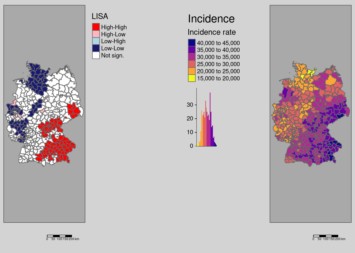
We can relate this to the Moran’s scatterplot:
mPlotRes <- moran.plot(ebiMc$z,
           listw = unionedListw_d,
           return_df=TRUE, plot=FALSE)

mPlotRes$localM <- covidKreise$localM

ggplot(data= mPlotRes, aes(x=x, y=wx, col=localM)) +
  geom_point() +
  geom_hline(yintercept = mean(mPlotRes$wx), lty=2)+
  geom_vline(xintercept = mean(mPlotRes$x), lty=2) +
  annotate(geom="label", x=1.5, y=1.5,
           label="high-high", col="red") +
  annotate(geom="label", x=-1.5, y=-1.5,
           label="low-low", col="midnightblue") +
  annotate(geom="label", x=1.5, y=-1.5,
           label="high-low", col="lightpink") +
    annotate(geom="label", x=-1.5, y=1.5,
           label="low-high", col="lightblue") +
  xlab("EBI") + ylab("EBI lagged") +
  labs(title="Germany, COVID-19",
       subtitle = "Cases till 28.04.2022") +
   scale_color_manual(values = localMcPalette, name="local Moran's I")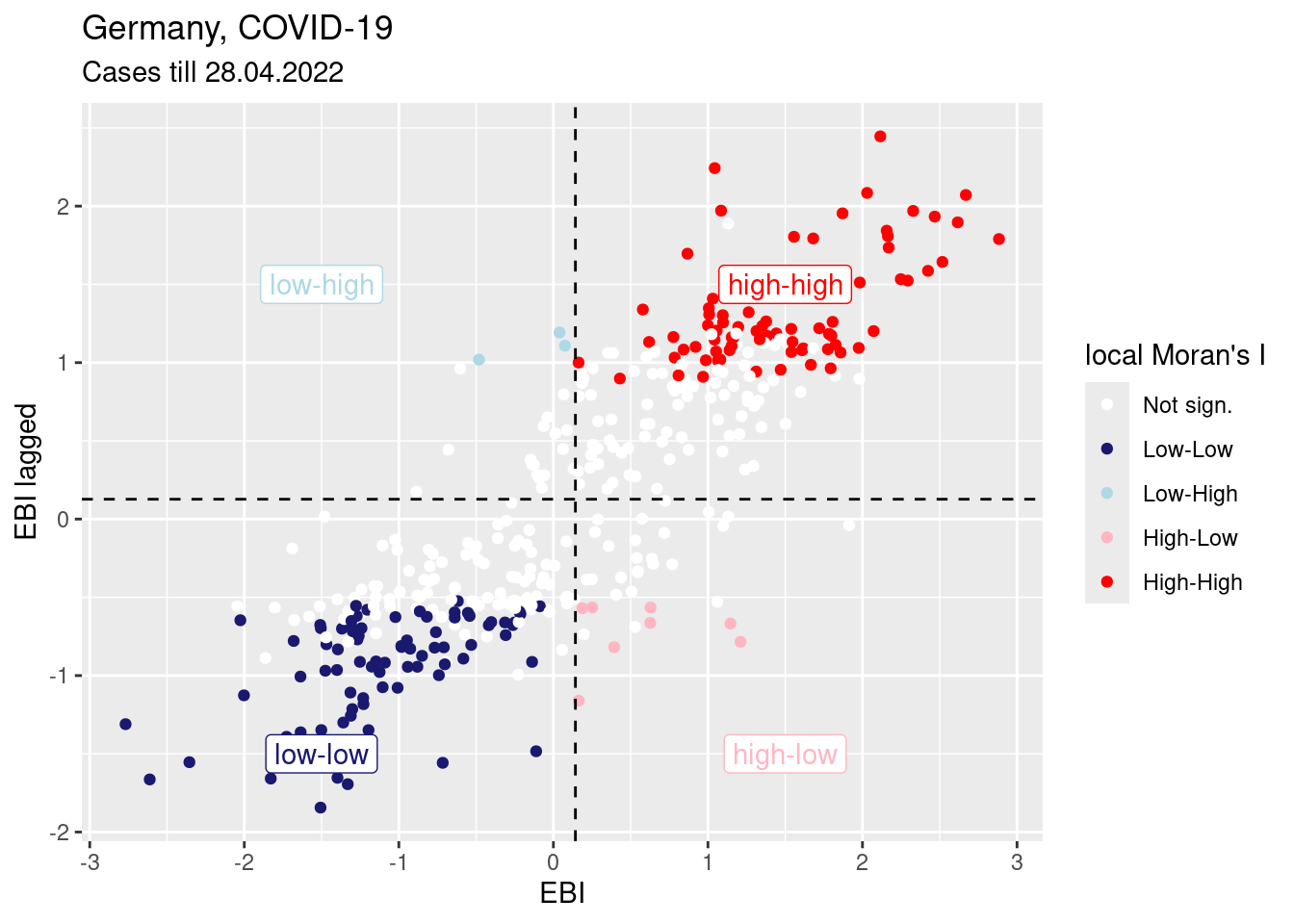
As Moran’s I can be interpreted as the slope of the regression line in the Moran scatterplot it might be interesting to determine the leverage of the different observations on the regression line between \(Wx\) and \(x\). These are shown in the next plot by the size of the dots in the scatterplot. The usual threshold would be \(2k/n\) with \(k\) the number of parameters in the regression model, which is here 2 (intercept and coefficient for \(x\)) and \(n\) the number of observations. The threshold is here: 0.01
mPlotRes$cooksdist <- cooks.distance(lm(wx ~x, data= mPlotRes))
mPlotRes$leverage <- lm.influence(lm(wx ~x, data= mPlotRes))$hat
mPlotRes$leverageAboveThreshold <- ifelse(mPlotRes$leverage > 4/ nrow(mPlotRes), "above", "below")

ggplot(data= mPlotRes, aes(x=x, y=wx, col=leverageAboveThreshold, size=leverage)) +
  geom_point() +
  geom_hline(yintercept = mean(mPlotRes$wx), lty=2)+
  geom_vline(xintercept = mean(mPlotRes$x), lty=2) +
  geom_smooth(data= mPlotRes, mapping= aes(x=x, y=wx),
              inherit.aes = FALSE, method="lm",
              col="black") +
  annotate(geom="label", x=1.5, y=1.5,
           label="high-high", col="red") +
  annotate(geom="label", x=-1.5, y=-1.5,
           label="low-low", col="midnightblue") +
  annotate(geom="label", x=1.5, y=-1.5,
           label="high-low", col="lightpink") +
    annotate(geom="label", x=-1.5, y=1.5,
           label="low-high", col="lightblue") +
  xlab("EBI") + ylab("EBI lagged") +
  labs(title="Germany, COVID-19",
       subtitle = "Cases till 28.04.2022") +
   scale_color_manual(values = c("black", "grey"), name="leverage threshold")
## `geom_smooth()` using formula = 'y ~ x'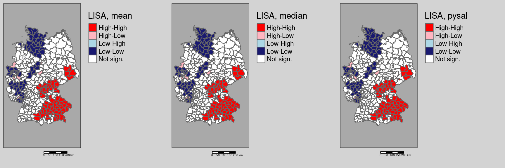
We see that around two dozens districts have a large pull and influence the value of global Moran’s I. However, we also see that these are not outliers since the regression line would not change drastically if these points would be eliminated.
We can also highlight the districts with a high leverage in the Moran scatterplot in the map:
m1 +
  tm_shape(covidKreise[mPlotRes$leverageAboveThreshold == "above",]) +
  tm_borders(col="black", lwd = 2)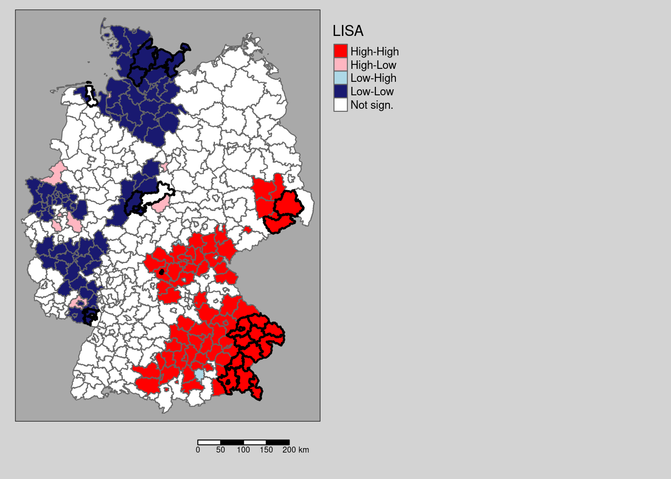
Let’s have a look on how the other two ways of defining the labels would change results:
covidKreise$localMmedian <- getLocalMoranFactor(ebiMc$z, listw = unionedListw_d, pval=0.05, quadr = "median")
covidKreise$localMpysal <- getLocalMoranFactor(ebiMc$z, listw = unionedListw_d, pval=0.05, quadr = "pysal")
titleSize <- .8
m1 <- tm_shape(covidKreise) +
tm_polygons(fill="localM",
fill.scale= tm_scale_categorical(values= localMcPalette),
fill.legend= tm_legend(title = "Local Moran's I",
reverse=TRUE)
) +
tm_layout(legend.outside = TRUE, bg.color = "darkgrey", outer.bg.color = "lightgrey",
legend.outside.size = 0.5, attr.outside = TRUE,
legend.outside.position = "right") +
tm_scalebar(position = tm_pos_auto_out()) +
tm_title(text="Option mean", size = titleSize)
m2 <- tm_shape(covidKreise) +
tm_polygons(fill="localMmedian",
fill.scale= tm_scale_categorical(values= localMcPalette),
fill.legend= tm_legend(title = "Local Moran's I",
reverse=TRUE)
) +
tm_layout(legend.outside = TRUE, bg.color = "darkgrey", outer.bg.color = "lightgrey",
legend.outside.size = 0.5, attr.outside = TRUE,
legend.outside.position = "right") +
tm_scalebar(position = tm_pos_auto_out()) +
tm_title(text="Option median", size = titleSize)
m3 <- tm_shape(covidKreise) +
tm_polygons(fill="localMpysal",
fill.scale= tm_scale_categorical(values= localMcPalette),
fill.legend= tm_legend(title = "Local Moran's I",
reverse=TRUE)
) +
tm_layout(legend.outside = TRUE, bg.color = "darkgrey", outer.bg.color = "lightgrey",
legend.outside.size = 0.5, attr.outside = TRUE,
legend.outside.position = "right") +
tm_scalebar(position = tm_pos_auto_out()) +
tm_title(text="Option pysal", size = titleSize)
tmap_arrange(m1, m2, m3)
For this data set no differences are present.
Testing different ways of adjusting for multiple testing
covidKreise$localMnone <- getLocalMoranFactor(ebiMc$z, listw = unionedListw_d, pval=0.05, p.adjust.method = "none")
covidKreise$localMbonf <- getLocalMoranFactor(ebiMc$z, listw = unionedListw_d, pval=0.05, p.adjust.method = "bonferroni")
m1 <- tm_shape(covidKreise) +
tm_polygons(fill="localM",
fill.scale= tm_scale_categorical(values= localMcPalette),
fill.legend= tm_legend(title = "Local Moran's I",
reverse=TRUE)
) +
tm_layout(legend.outside = TRUE, bg.color = "darkgrey", outer.bg.color = "lightgrey",
legend.outside.size = 0.5, attr.outside = TRUE,
legend.outside.position = "right") +
tm_scalebar(position = tm_pos_out()) +
tm_title(text="Holm correction", size = titleSize)
m2 <- tm_shape(covidKreise) +
tm_polygons(fill="localMnone",
fill.scale= tm_scale_categorical(values= localMcPalette),
fill.legend= tm_legend(title = "Local Moran's I",
reverse=TRUE)
) +
tm_layout(legend.outside = TRUE, bg.color = "darkgrey", outer.bg.color = "lightgrey",
legend.outside.size = 0.5, attr.outside = TRUE,
legend.outside.position = "right") +
tm_scalebar(position = tm_pos_out()) +
tm_title(text="Without correction", size = titleSize)
m3 <- tm_shape(covidKreise) +
tm_polygons(fill="localMbonf",
fill.scale= tm_scale_categorical(values= localMcPalette),
fill.legend= tm_legend(title = "Local Moran's I",
reverse=TRUE)
) +
tm_layout(legend.outside = TRUE, bg.color = "darkgrey", outer.bg.color = "lightgrey",
legend.outside.size = 0.5, attr.outside = TRUE,
legend.outside.position = "right") +
tm_scalebar(position = tm_pos_out()) +
tm_title(text="Bonferoni correction", size = titleSize)
tmap_arrange(m1, m2, m3)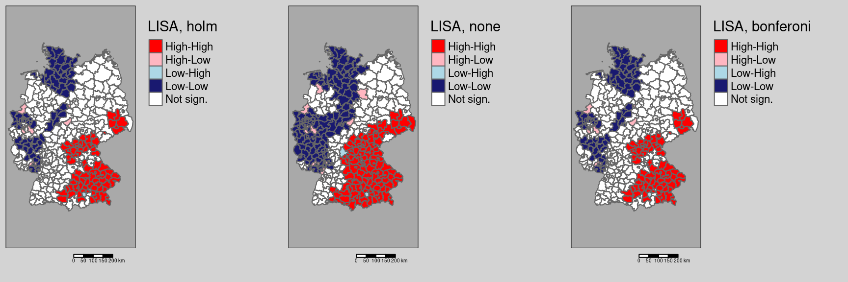
As we see, there are remarkable differences. Not correction for multiple testing leads to a large number of districts with significant local spatial autocorrelation: We see a clear spatial pattern: the South-East (Bavaria, Saxony, parts of Baden-Württemberg) is characterized by districts with high values compared to the global mean which are surrounded by similar values (high positive autocorrelation). Large parts of Rhineland-Palatina, NRW, Schleswig-Holstein and parts of Lower Saxony have low incidence rates (compared to the global mean) and are surrounded by districts with dissimilar incidence rates. This region is characterized by strong differences between the different districts. In between we always see a few districts that are spatial outliers.
The correction by Holm renders many of those districts non significant (cf. 9.1). For this example, no differences exist between the conservative Bonferoni and the Holm correction with respect to the districts labeled as significant.
# which districts are no longer significant?
covidKreiseDiffPvalClassNoneBonferoni <- filter(covidKreise, localMnone != "Not sign." & localMbonf == "Not sign.")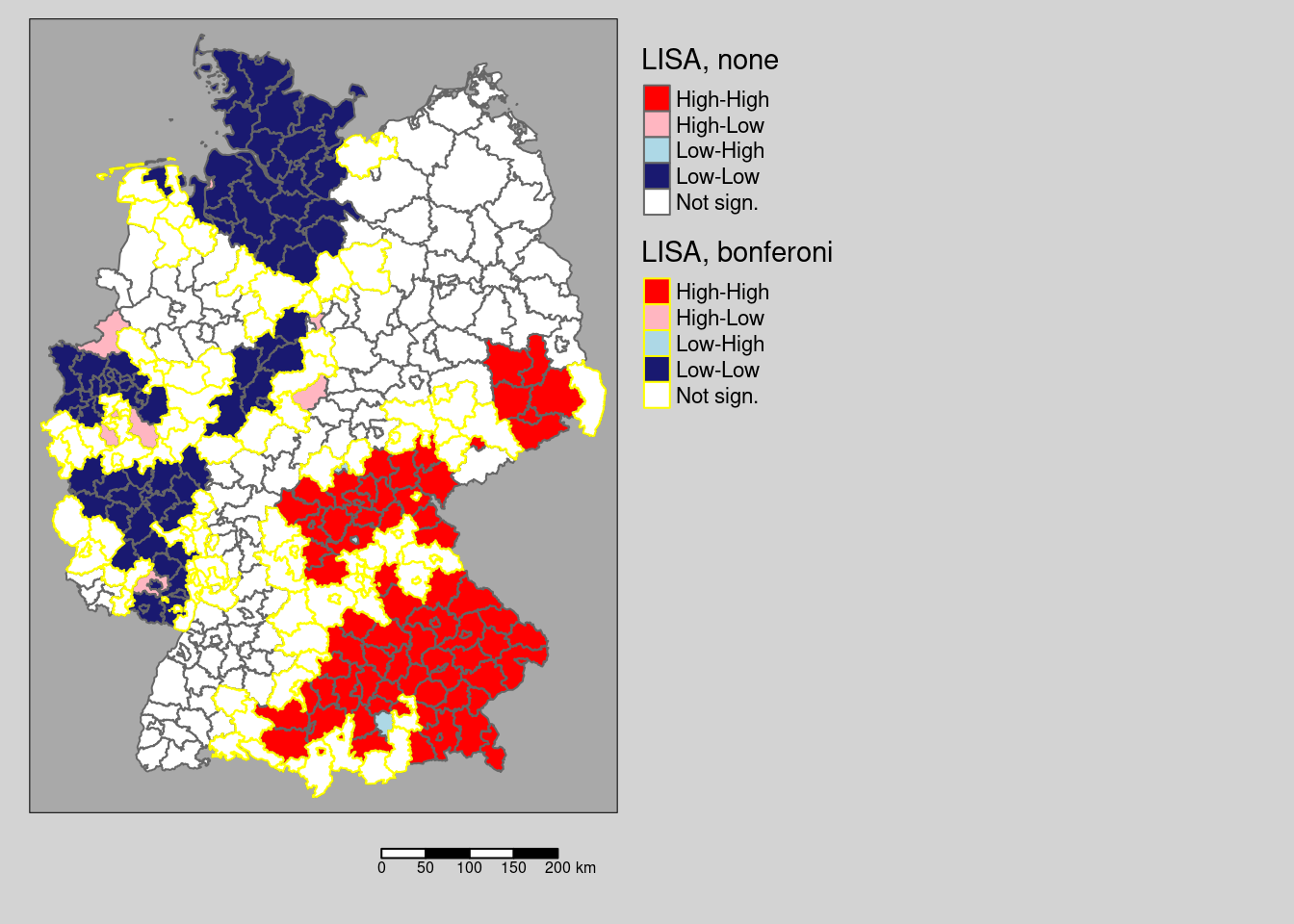
Figure 9.1: Changes in significance for the test based on a normal approximation. The regions highlighted by a yellow outline are those that are significant without p-value adjustment compared to a Bonferoni adjustment. For this example there is no difference between the districts labeld as significant for the Holm and the Bonferoni correction.
Comparing permutation test results with the normal approximation test:
covidKreise$localMperm <- getLocalMoranFactor(ebiMc$z, listw = unionedListw_d,
                                              pval=0.05, p.adjust.method = "holm",
                                              method = "perm", nsim=9999)
m1 <- tm_shape(covidKreise) +
tm_polygons(fill="localM",
fill.scale= tm_scale_categorical(values= localMcPalette),
fill.legend= tm_legend(title = "Local Moran's I",
reverse=TRUE)
) +
tm_layout(legend.outside = TRUE, bg.color = "darkgrey", outer.bg.color = "lightgrey",
legend.outside.size = 0.5, attr.outside = TRUE,
legend.outside.position = "right") + tm_scalebar(position = tm_pos_out()) +
tm_title(text="Normal approx.", size = titleSize)
m2 <- tm_shape(covidKreise) +
tm_polygons(fill="localMperm",
fill.scale= tm_scale_categorical(values= localMcPalette),
fill.legend= tm_legend(title = "Local Moran's I",
reverse=TRUE)
) +
tm_layout(legend.outside = TRUE, bg.color = "darkgrey", outer.bg.color = "lightgrey",
legend.outside.size = 0.5, attr.outside = TRUE,
legend.outside.position = "right") + tm_scalebar(position = tm_pos_out()) +
tm_title(text="Permutation test", size = titleSize)
tmap_arrange(m1, m2)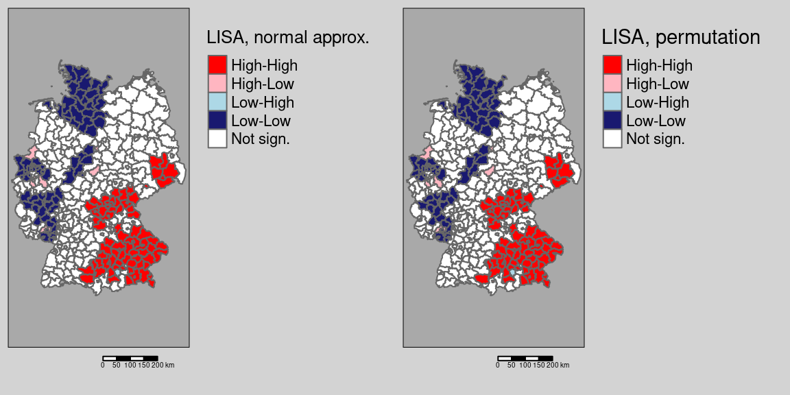
We see a few differences, e.g. on district in the cluster in Saxony is no longer significant based on the (presumably more correct) permutation test. We filter those districts that change from significant \(I_i\) to not significant between the two and map them (cf. figure 9.2).
# which districts are no longer significant?
covidKreiseDiffPvalClass <- filter(covidKreise, localM != "Not sign." & localMperm == "Not sign.")

covidKreiseDiffPvalClass$GEN
## [1] "Solingen" "Köln" "Euskirchen" "Lahn-Dill-Kreis"
## [5] "Greiz"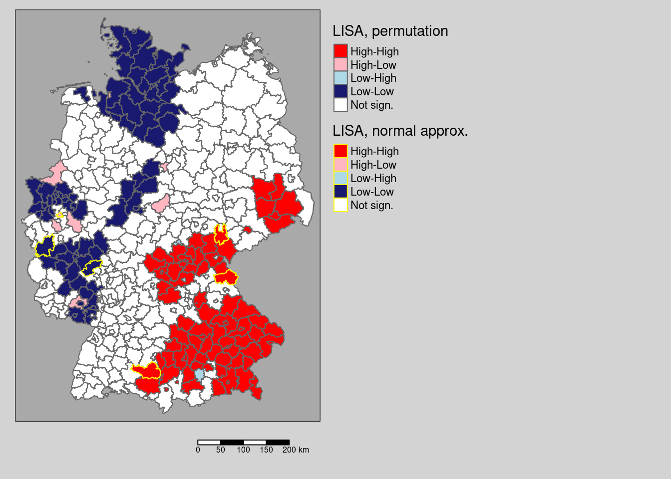
Figure 9.2: Changes in significance for the test based on a normal approximation and for a permuation test with 999 replications. The regions highlighted by a yellow outline are those that are significant for the normal approximation, but not based on the permutation test.
9.3.2 Local Geary’s C
For comparison we calculate Geary’s C, that is based on the squared differences between neighboring observations instead of the product of their differences of the mean. We did not provide a convenience function but the code is relatively straight forward. We calculate local Geary’s C using the parametric test or the permutation test (the later as usual recommended), extract the p-values, which are stored as an attribute of the returned object and adjust those for multiple testing (using the approach by Holm). We use that to filter for non-significant districts which are used as a mask then we creat the map. The information about the quadrants (named differently compared to local Moran’s I) is as well stored in an attribute that we extract with attr(object, nameOfTheAttribute). attributes(object) would return us all attributes of an object.
covidKreise$Gc <- localC(ebiMc$z, listw = unionedListw_d)

locGc <- localC_perm(ebiMc$z, listw = unionedListw_d, nsim = 9999)
covidKreise$GcPval <- attr(locGc, "pseudo-p")[,5]
covidKreise$GcPval <- p.adjustSP(covidKreise$GcPval,
                                 nb = unionedListw_d$neighbours, method = "holm")
covidKreiseGcPval_nonsignif <- filter(covidKreise, GcPval > 0.05)
covidKreise$GcQuadr <- attr(locGc, "cluster")
#unique(covidKreise$GcQuadr)
localCPalette <- rev(c("lightblue", "lightpink", "midnightblue", "red"))
tm_shape(covidKreise, is.master = TRUE) +
tm_polygons(fill="GcQuadr",
fill.scale= tm_scale_categorical(values= localCPalette),
fill.legend= tm_legend(title = "Local Geary's C",
reverse=TRUE)
) +
tm_shape(covidKreiseGcPval_nonsignif) +
tm_fill(fill=tm_const(), fill_alpha=0.7) +
tm_layout(legend.outside = TRUE, bg.color = "darkgrey", outer.bg.color = "lightgrey",
legend.outside.size = 0.5, attr.outside = TRUE,
legend.outside.position = "right") + tm_scalebar(position = tm_pos_out())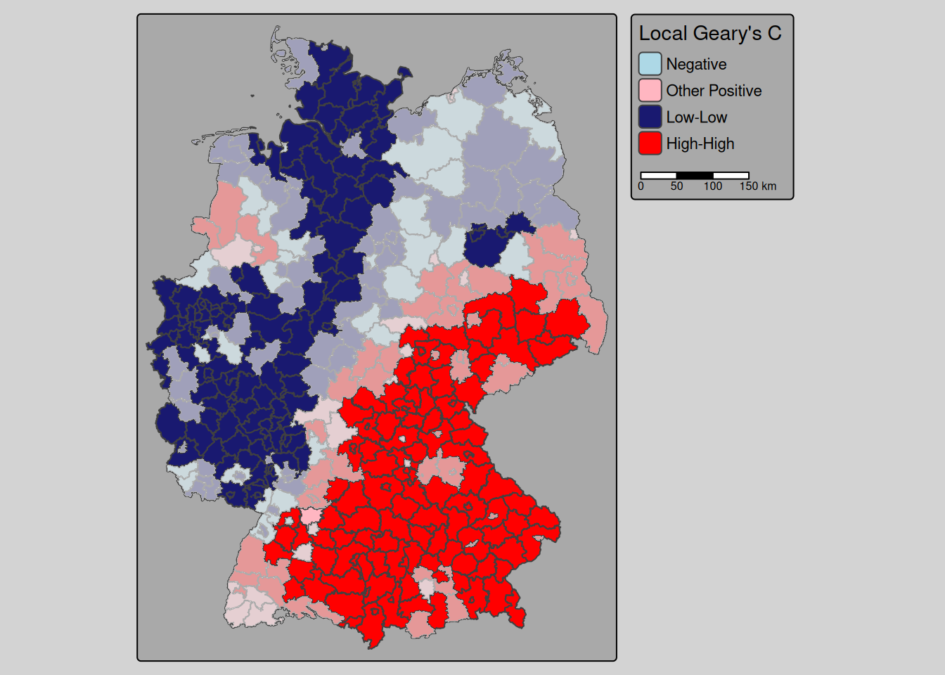
Figure 9.3: Local Geary’s C for the empirical bayes index of the incidence cases. Non significant districts are overlayed with a semi-transparent mask.
The pattern is similar to the map for local Moran’s I with some differences. Chemnitz for example does not show up as a high-high cluster by Geary’s C but Berlin and Brandenburg an der Havel were identified by Geary’s C but not by Moran’s I as part of a low-low cluster. Geary’s C high-high cluster reaches much far to south western Baden-Württemberg and the low-low cluster in NRW, norhtern Rhineland-Palatina differs between the two approaches. Hamburg is part of the low-low cluster in Moran’s I but not for Geary’s C. The differences might however look more pronounced than they are due to the cutoff value used for the significance testing.
The map shown above is based on the permutation test, but the similar approach could be used for the parametric test.
9.3.3 Getis G and Gstar
Both localG and localG_perm return a z-score that indicates the probability of observing such a value by chance (expressed in terms of the standard normal distribution so usual thresholds are valid).
covidKreise$Gi <- localG(ebiMc$z, listw = unionedListw_d)
covidKreise$Gi_perm <- localG_perm(ebiMc$z, listw = unionedListw_d, nsim = 999)
#covidKreiseGiPval_nonsignif <- filter(covidKreise, abs(Gi_perm) < 1.96)
Classify values with respect to the probability:
breaks <- c(min(covidKreise$Gi_perm ), -2.58, -1.96, -1.65, 1.65, 1.96, 2.58, max(covidKreise$Gi_perm ))

covidKreise <- covidKreise %>% mutate(gCluster = cut(Gi_perm, breaks=breaks, include.lowest = TRUE, labels=c("Cold spot: 99% confidence", "Cold spot: 95% confidence", "Cold spot: 90% confidence", "Not significant","Hot spot: 90% confidence", "Hot spot: 95% confidence", "Hot spot: 99% confidence"))) tm_shape(covidKreise) +
tm_polygons(fill="gCluster",
fill.scale= tm_scale_categorical(values= "-brewer.rd_bu"),
fill.legend= tm_legend(title = "Local Getis G",
reverse=TRUE)
) +
tm_layout(legend.outside = TRUE, bg.color = "darkgrey", outer.bg.color = "lightgrey",
legend.outside.size = 0.5, attr.outside = TRUE,
legend.outside.position = "right") +
tm_scalebar(position= tm_pos_out())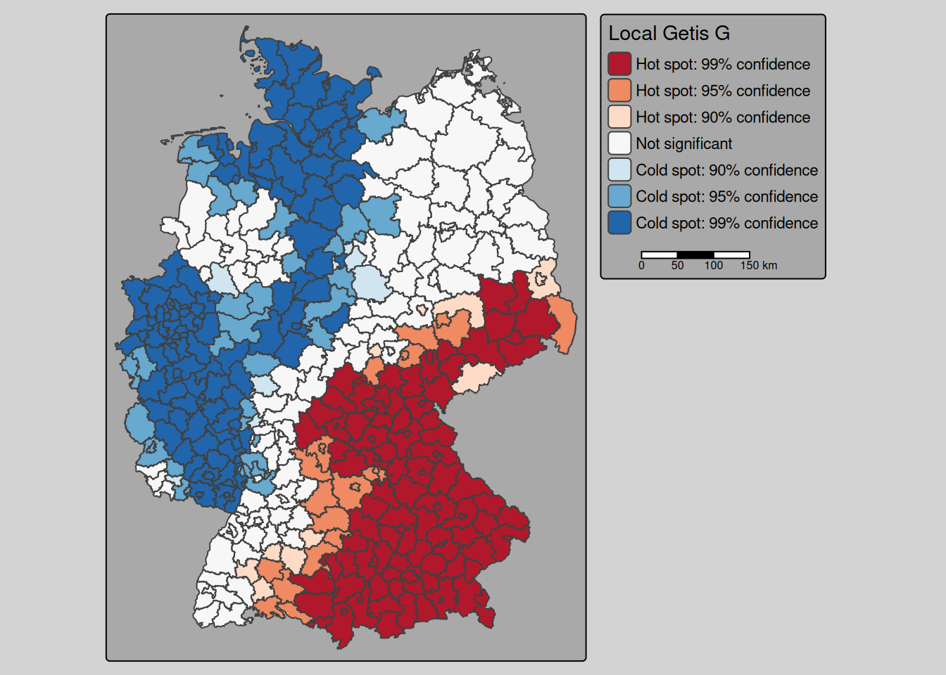
Getis G indicates a clear separation in a belt of high values in Bavaria, Saxony and parts ofThuringia and Baden-Württemberg and a cold spot belt in most of NRW, Rhineland-Palatino, Schleswig-Holstein and parts of Lower Saxony.
For Getis G* we need to create a new weighted list including the observation itself. This makes it impossible to use inverse distance weighting as it includes a distance of zero.
unionedListw_self <-  nb2listw(include.self(unionedNb), style = "W")

covidKreise$GiStar <- localG(ebiMc$z, listw = unionedListw_self)
covidKreise$GiStar_perm <- localG_perm(ebiMc$z, listw = unionedListw_self, nsim = 999)
breaks <- c(min(covidKreise$GiStar_perm ), -2.58, -1.96, -1.65, 1.65, 1.96, 2.58, max(covidKreise$GiStar_perm ))
covidKreise <- covidKreise %>% mutate(gStarCluster = cut(GiStar_perm, breaks=breaks, include.lowest = TRUE, labels=c("Cold spot: 99% confidence", "Cold spot: 95% confidence", "Cold spot: 90% confidence", "Not significant","Hot spot: 90% confidence", "Hot spot: 95% confidence", "Hot spot: 99% confidence"))) tm_shape(covidKreise) +
tm_polygons(fill="gStarCluster",
fill.scale= tm_scale_categorical(values= "-brewer.rd_bu"),
fill.legend= tm_legend(title = "Local Getis G*",
reverse=TRUE)
) +
tm_layout(legend.outside = TRUE, bg.color = "darkgrey", outer.bg.color = "lightgrey",
legend.outside.size = 0.5, attr.outside = TRUE,
legend.outside.position = "right") + tm_scalebar()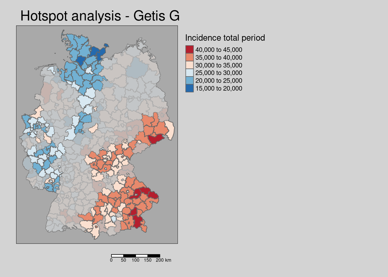
While absolute values change slightly, the overall pattern for G* is similar with a few exceptions as for G.
The maps we have created so far are not adjusted for the multiple testing problem. The function localG_perm returns an attribute called internals with intermediate results that could be used to account for this.
Gi_perm_internals <- attr(covidKreise$Gi_perm, "internals") %>%
  as.data.frame()
names(Gi_perm_internals)
## [1] "Gi" "E.Gi" "Var.Gi"
## [4] "StdDev.Gi" "Pr(z != E(Gi))" "Pr(z != E(Gi)) Sim"
## [7] "Pr(folded) Sim" "Skewness" "Kurtosis"Next we extract the field “Pr(folded) Sim” with contains the simulation based p-value and adjust that for the multiple testing problem using Holm’s approach. The use p.adjustSP that only takes the number of neighbors for each unit as the factor to be included (instead of taking the total number of spatial units which would be too conservative). Based on that we create a polygon mask that we will plot on top of Getis G values.
covidKreise$Gi_perm_padj <- p.adjustSP(p= Gi_perm_internals[, "Pr(folded) Sim"], nb = unionedNb, method = "holm")
covidKreise_Gi_permNonSignifSf <- filter(covidKreise, Gi_perm_padj > 0.05)tm_shape(covidKreise) +
tm_polygons(fill="Gi_perm",
fill.scale= tm_scale_intervals(values= "-brewer.rd_bu", midpoint= 0),
fill.legend= tm_legend(title = "Local Getis G, p-values, Holm",
reverse=TRUE)
) +
tm_shape(covidKreise_Gi_permNonSignifSf) + tm_fill(fill="grey", fill_alpha=.7) +
tm_layout(legend.outside = TRUE, bg.color = "darkgrey", outer.bg.color = "lightgrey",
legend.outside.size = 0.5, attr.outside = TRUE,
legend.outside.position = "right") +
tm_scalebar(position = tm_pos_out())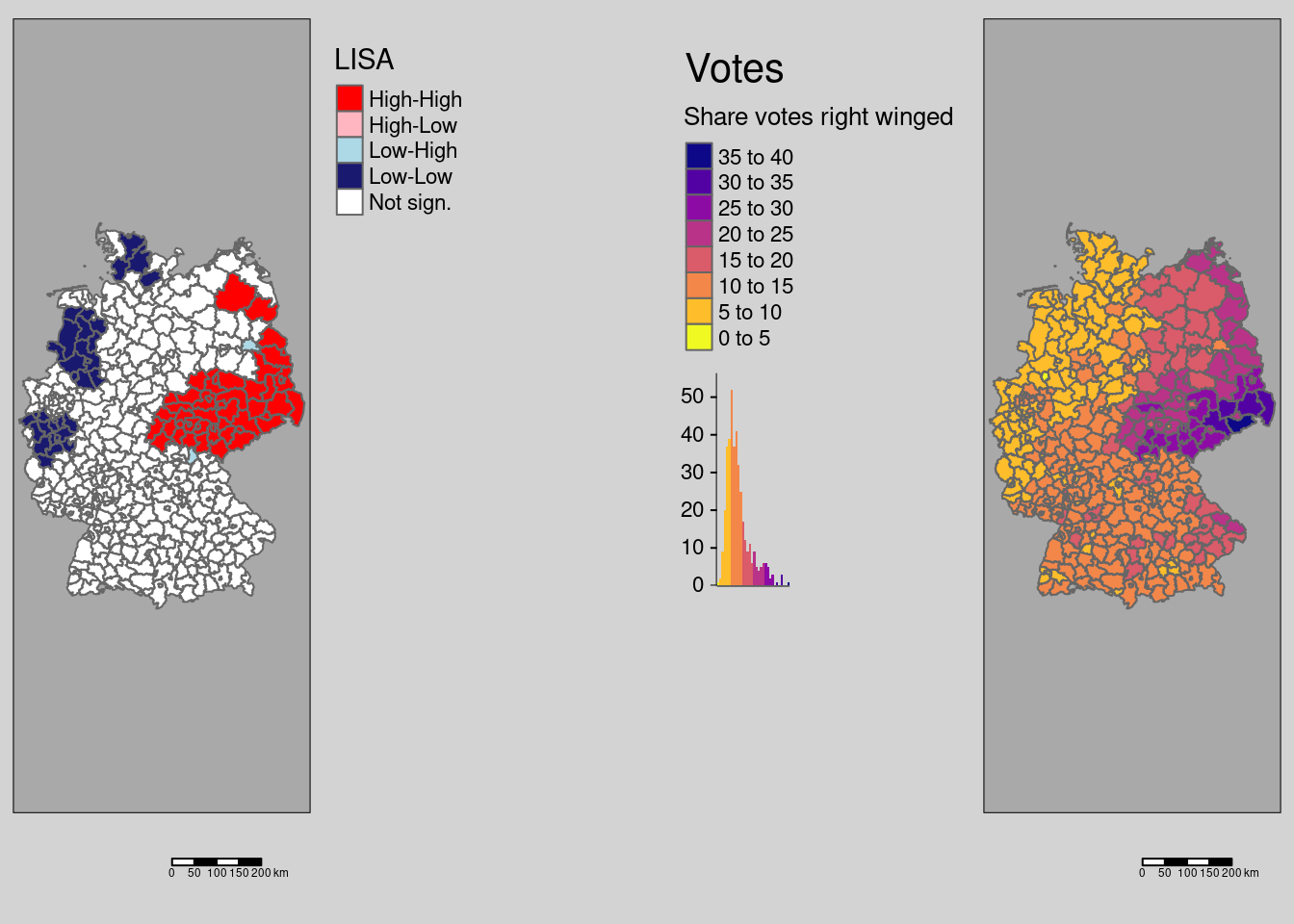
The map shows the Getis G values all areas, that are non significant after holm correction are masked.
We could as well plot the incidence rate and use the Getis G based mask.
tm_shape(covidKreise) +
  tm_polygons(fill="incidenceTotal",
              fill.scale= tm_scale_intervals(values=  "brewer.reds"),
              fill.legend= tm_legend(title = "Incidence total period",
                                                reverse=TRUE)
             ) +
  tm_shape(covidKreise_Gi_permNonSignifSf) +
  tm_fill(fill="grey", fill_alpha=.8) +
  tm_layout(legend.outside = TRUE, bg.color = "darkgrey", outer.bg.color = "lightgrey",
            legend.outside.size = 0.5, attr.outside = TRUE,
            legend.outside.position = "right") +
  tm_scalebar(position = tm_pos_out()) +
  tm_title( "Hotspot analysis - Getis G mask")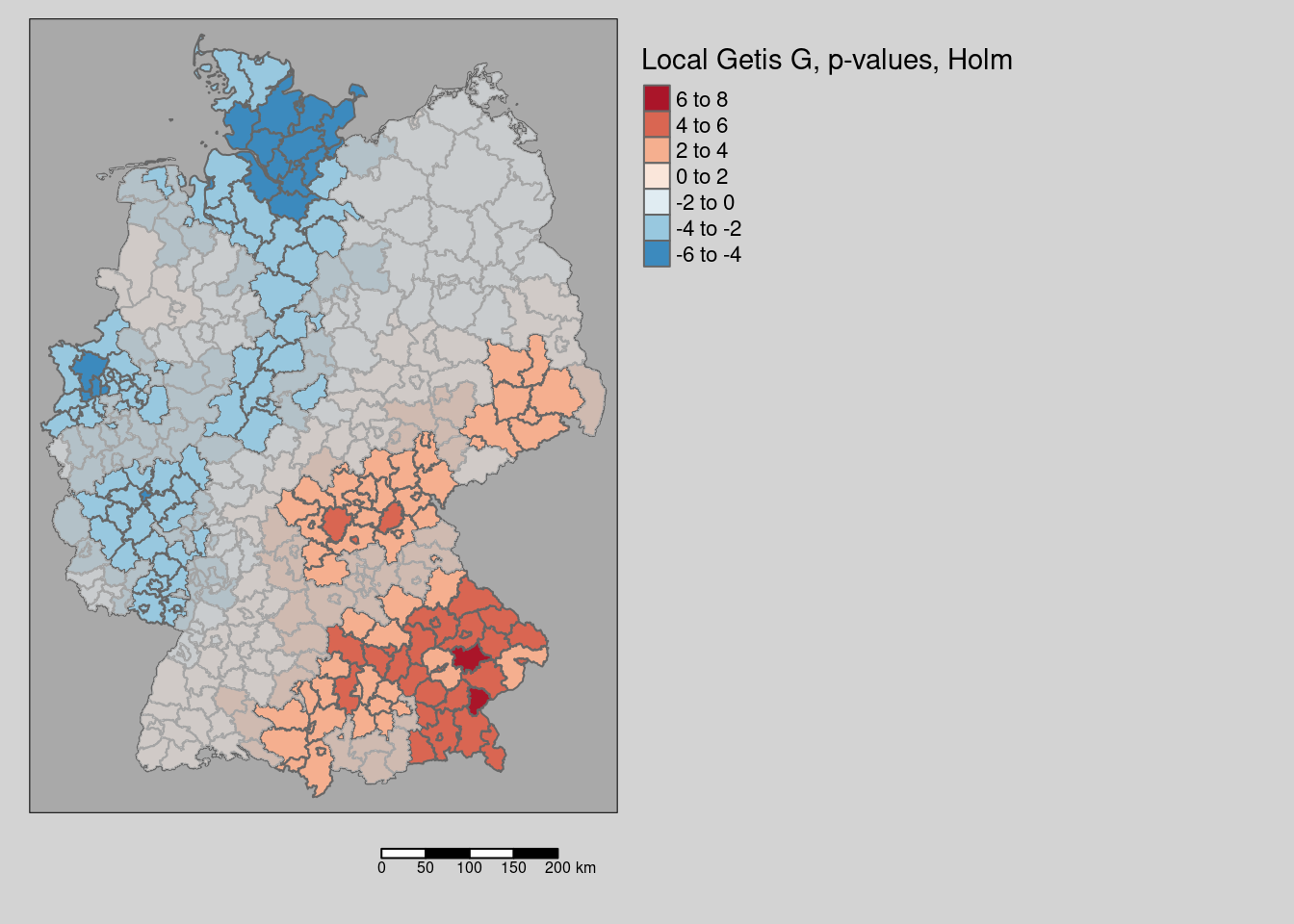
9.3.4 Lee’s L
lee returns not only the global but also the local Lee’s L - unfortunately without p-values5. We are here demonstrating the simple use at the example of the empirical bayes index of the COVID-19 incidence over the whole period and the votes at the last national election for the right winged party (AfD).
covidKreise$localL_ebi_AfD <- lee(ebiMc$z, covidKreise$Stimmenanteile.AfD,
    listw = unionedListw_d,
n=nrow(covidKreise))$localLtm_shape(covidKreise) +
tm_polygons(fill="localL_ebi_AfD",
fill.scale= tm_scale_intervals(values= "brewer.rd_bu",
breaks=c(-2, -.75, -.5, -.25, 0, .25, .5, .75, 6),
midpoint =0),
fill.legend= tm_legend(title = "Local Lee's L",
reverse=TRUE)
) +
tm_layout(legend.outside = TRUE, bg.color = "darkgrey", outer.bg.color = "lightgrey",
legend.outside.size = 0.5, attr.outside = TRUE,
legend.outside.position = "right") +
tm_scalebar(position = tm_pos_out()) +
tm_title("EBI Incidence total - votes AfD")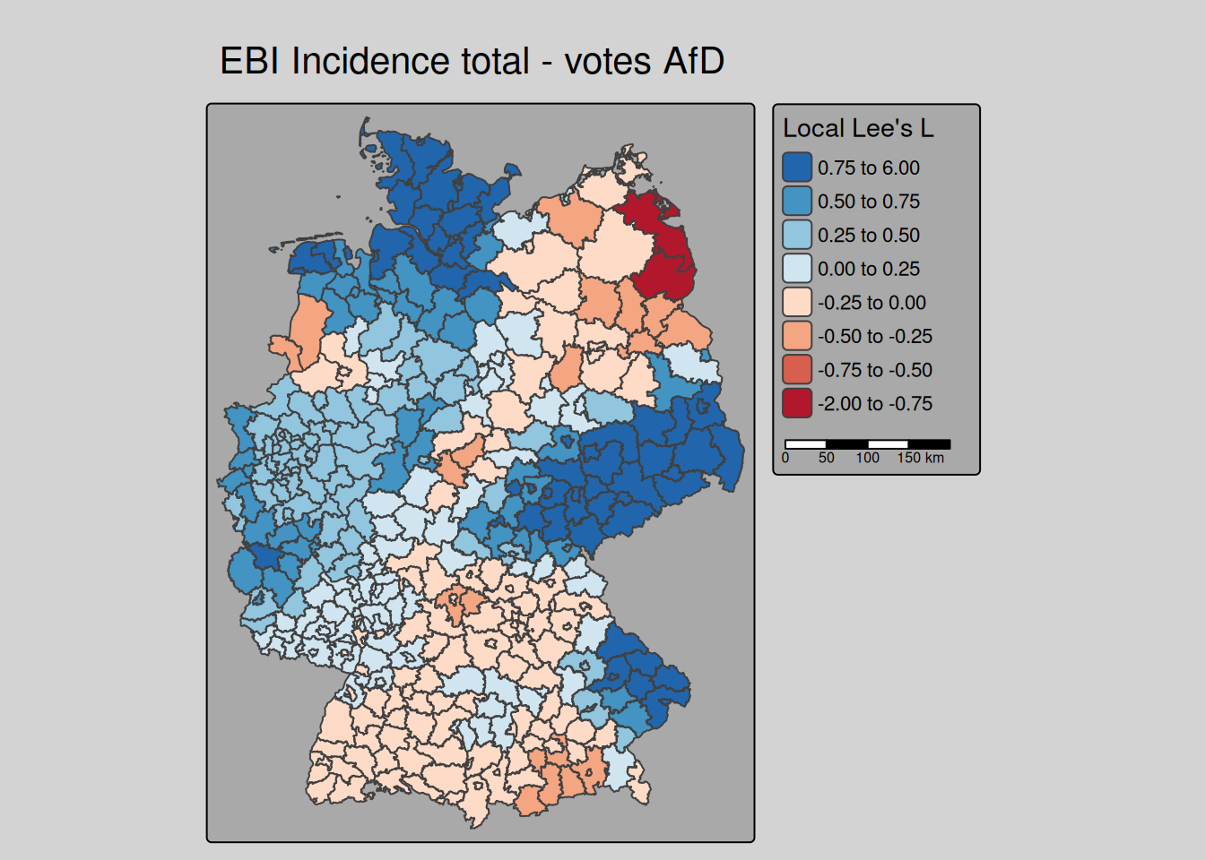
We see that for Saxony and neighboring parts of Brandenburg, Thuringia and Saxony-Anhalt as well as for Schleswig-Holstein and eastern Bavaria we have a strong positive association. To bit lower degree for large parts of NRW and Lower Saxony as well. For most of Bavaria and Baden-Württemberg we have no or a negative (dissimilar pattern) bivariate spatial dependence between the COVID-19 indicende and the votes for the right winged party.
For comparison we show the incidence and the share of votes for the right winged party maps again.
covm1 <- tm_shape(covidKreise) +
  tm_polygons(fill="Stimmenanteile.AfD",
              fill.scale= tm_scale_intervals(values=  "brewer.blues"),
              fill.legend= tm_legend(title = "Share votes",
                                                reverse=TRUE)
              ) +
  tm_layout(legend.outside = TRUE, bg.color = "darkgrey", outer.bg.color = "lightgrey",
            legend.outside.size = 0.5, attr.outside = TRUE,
            legend.outside.position = "left") +
  tm_scalebar(position = tm_pos_out()) +
  tm_title("Rightwinged votes")

covm2 <- tm_shape(covidKreise) +
  tm_polygons(fill="incidenceTotal",
              fill.scale= tm_scale_intervals(values=  "-plasma"),
              fill.legend= tm_legend(title = "Incidence rate",
                                                reverse=TRUE)
              ) +
  tm_layout(legend.outside = TRUE, bg.color = "darkgrey", outer.bg.color = "lightgrey",
            legend.outside.size = 0.5, attr.outside = TRUE,
            legend.outside.position = "right") +
  tm_scalebar(position = tm_pos_out()) +
  tm_title("COVID-19 till 28.04.2022")

tmap_arrange(covm1, covm2)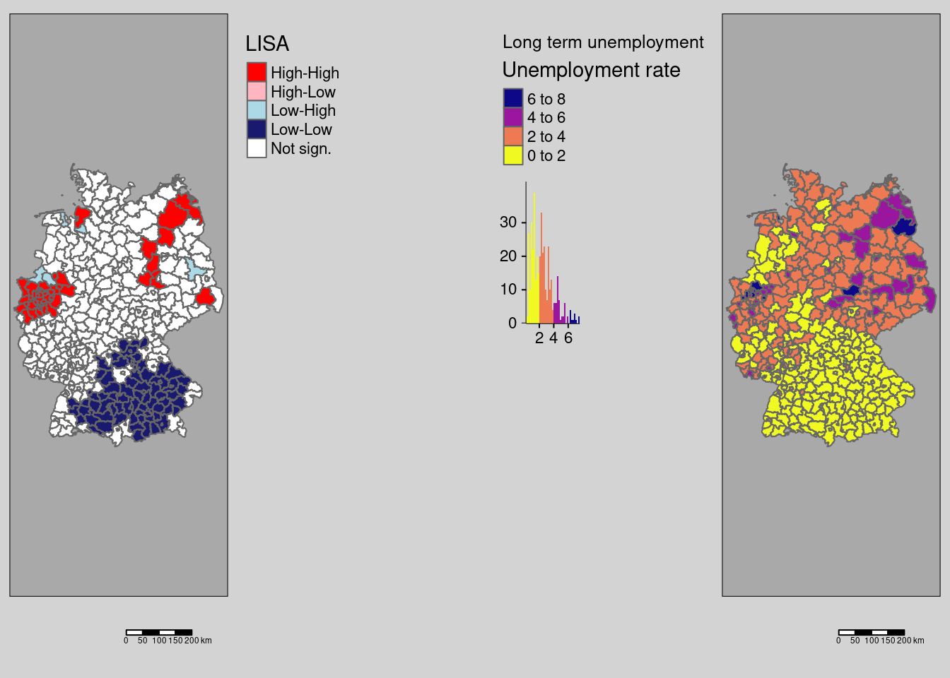
To estimate the p-values, we use a simple non-parametric bootstrap approach together with the Holm adjustment for multiple testing
simula_lee <- function(x, y, listw, nsim = 999,
                       alpha=0.05, alternative = "two.sided",
                       p.adjust.method ="holm",
                       zero.policy = NULL, na.action = na.fail) {
  alternative <- match.arg(alternative, c("greater", "less",
        "two.sided"))
  if (deparse(substitute(na.action)) == "na.pass")
    stop ("na.pass not permitted")
  na.act <- attr(na.action(cbind(x, y)), "na.action")
  x[na.act] <- NA
  y[na.act] <- NA
  x <- na.action(x)
  y <- na.action(y)
  if (!is.null(na.act)) {
    subset <- !(1:length(listw$neighbours) %in% na.act)
    listw <- subset(listw, subset, zero.policy = zero.policy)
  }
  n <- length(listw$neighbours)
  if ((n != length(x)) | (n != length(y)))
    stop ("objects of different length")
  gamres <- suppressWarnings(nsim > gamma(n + 1))
  if (gamres)
    stop ("nsim too large for this number of observations")
  if (nsim < 1)
    stop ("nsim too small")
  xy <- data.frame(x, y)
  S2 <- sum((unlist(lapply(listw$weights, sum)))^2)


  boot_res <- matrix(nrow=n, ncol = nsim + 1)

 for (j in 1:nsim)
   {
   idx <- sample(1:n)
   boot_res[,j] <- lee(x[idx], y[idx], listw, n, S2, zero.policy)$localL
  }


  # estimates for local Lee's L
  m <- lee(x, y,
           listw = listw,n=n,
         zero.policy = zero.policy)
  boot_res[,nsim+1] <- m$localL

  xrank <- apply(boot_res, MARGIN = 1, function(x) rank(x)[nsim+1])

  posdiff <- nsim - xrank
  posdiff <- ifelse(posdiff > 0, posdiff, 0)

  if (alternative == "less") {
    pval <- punif((posdiff + 1)/(nsim + 1), lower.tail = FALSE)
  } else if (alternative == "greater") {
    pval <- punif((posdiff + 1)/(nsim + 1))
  } else pval <- punif(abs(xrank - (nsim + 1)/2)/(nsim + 1),
        0, 0.5, lower.tail = FALSE)

  if (any(!is.finite(pval)) || any(pval < 0) || any(pval > 1))
        warning("Out-of-range p-value: reconsider test arguments")
  # adjustment for multiple testing
  pval <- p.adjustSP(pval, nb = listw$neighbours,
                     method=p.adjust.method)

  res <- list(localL = m$localL, p.val = pval)
  return(res)
}
# Local Lee's L simulations
local_sims <- simula_lee(ebiMc$z, covidKreise$Stimmenanteile.AfD,
listw = unionedListw_d, nsim = 9999,
zero.policy = TRUE, na.action = na.omit)We us the p-values to filter those districts with a non-significant local Lee’s L value and to mask them as before (cf. figure 9.4).
covidKreise$localL_ebi_AfD_pval <- local_sims$p.val

covidKreise_localL_ebi_AfD_nonsig <- filter(covidKreise, localL_ebi_AfD_pval > 0.05)tm_shape(covidKreise) +
tm_polygons(fill="localL_ebi_AfD",
fill.scale= tm_scale_intervals(values= "-brewer.rd_bu",
breaks=c(-2, -.75, -.5, -.25, 0, .25, .5, .75, 6),
midpoint =0),
fill.legend= tm_legend(title = "Local Lee's L",
reverse=TRUE)
) +
tm_shape(covidKreise_localL_ebi_AfD_nonsig) +
tm_fill(fill="grey", fill_alpha=.8) +
tm_layout(legend.outside = TRUE, bg.color = "darkgrey", outer.bg.color = "lightgrey",
legend.outside.size = 0.5, attr.outside = TRUE,
legend.outside.position = "right") +
tm_scalebar(position = tm_pos_out()) +
tm_title("EBI Incidence total - votes AfD")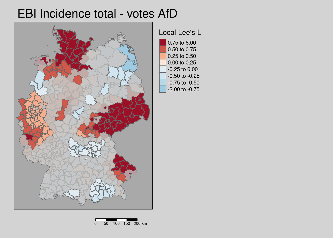
Figure 9.4: Local Lee’s L for the empirical Bayes index for the COVID-19 incidence till 28.04.2022. Non-significant areas are masked. Holm adjustment for p-values.
As we see a positive association between both variables is present for Saxony and neighboring parts of Brandenburg, Thuringia and Saxony-Anhalt as well as for Schleswig-Holstein, eastern Bavaria as well as for parts of NRW and Lower Saxony.
9.3.5 LOSH - local spatial heteroscedasticity
The LOSH considered local variances instead of local means. It can thereby be used to identify areas which contain both high and low values. These areas could represent transitional zones where different spatial processes overlap. This highlights of course areas different from the clusters identified by the other three local indicators of spatial autocorrelation as we are not interested in areas that are in a homogeneous neighborhood or are spatial outliers but in those there both high and low values are in a neighborhood.
The run LOSH on the empirical Bayes index derived before, using a permutation test. The method returns a matrix with four columns:
- Hi - the LOSH value for spatial unit i, \(H_i\)
- x_bar_i - the local spatial weighted mean for spatial unit i, \(\bar{x}_i\)
- ei - the residual about \(\bar{x}_i\) for spatial unit i, \(e_i\)
- Pr() - the p-value for \(H_i\)
For the formulas, see the theory section above.
We convert the matrix to a dataframe and bind it columnwise with the sf object - the order is the same, therefore we can simply cbind the two tables. The name of some colums in the matrix change as "P()" is not allowed for column names in a data.frame. Afterwards we adjust p-values for multiple testing using the spatial version p-adjustSP that considers only the number of neighbors of each object for the adjustment (same as for local Moran’s I, Geary’s C and Getis-Ord G or G*). The adjusted p-values are then used to filter the sf objects. The resulting sf objects is later used to mask non-significant areas then creating the map.
set.seed(3)
covidLosh <- LOSH.mc(ebiMc$z, listw = unionedListw_d, nsim = 499)
names(as.data.frame(covidLosh))
## [1] "Hi" "x_bar_i" "ei" "Pr()"covidKreiseLosh <- cbind(covidKreise, as.data.frame(covidLosh))
covidKreiseLosh$ebiMcZ <- ebiMc$z
# holm adjustment
covidKreiseLosh$pvalHiHolm <- p.adjustSP(covidKreiseLosh$Pr.., nb = unionedNb, method="holm")
covidKreiseLoshNoSign <- filter(covidKreiseLosh, pvalHiHolm> 0.1)Effect of the Holm adjustment for multiple testing:
##    Min. 1st Qu.  Median    Mean 3rd Qu.    Max.
## 0.0280 1.0000 1.0000 0.9322 1.0000 1.0000## Min. 1st Qu. Median Mean 3rd Qu. Max.
## 0.0020 0.2470 0.5580 0.5336 0.8340 0.9980As we see, for many districts \(H_i\) became not significantly differently from the expected value by the adjustment.
Next we plot the EBI, the LOSH (masking the non-significant districts by a semi-transparent layer). For a better understanding of the calculation of \(H_i\) we have added \(e_i\) and \(\bar{x}_i\) maps as well.
#tmap_mode("plot")
m1 <- tm_shape(covidKreiseLosh) +
  tm_polygons(fill="ebiMcZ",
              fill.scale= tm_scale_intervals(values=  "-brewer.rd_bu",
                                             midpoint = 0),
              fill.legend= tm_legend(title = "EBI, incidence",
                                                reverse=TRUE)
              ) +
  tm_layout(legend.outside = TRUE, bg.color = "darkgrey", outer.bg.color = "lightgrey",
            legend.outside.size = 0.5, attr.outside = TRUE,
            legend.outside.position = "right") +
  tm_scalebar(position = tm_pos_out())

m2 <- tm_shape(covidKreiseLosh) +
  tm_polygons(fill="Hi",
              fill.scale= tm_scale_intervals(values=  "brewer.reds"),
              fill.legend= tm_legend(title = "LOSH",
                                                reverse=TRUE)
              ) +
  tm_shape(covidKreiseLoshNoSign) +
  tm_fill(fill="grey", fill_alpha = 0.8) +
  tm_layout(legend.outside = TRUE, bg.color = "darkgrey", outer.bg.color = "lightgrey",
            legend.outside.size = 0.5, attr.outside = TRUE,
            legend.outside.position = "right") +
   tm_scalebar(position = tm_pos_out())

m3 <- tm_shape(covidKreiseLosh) +
  tm_polygons(fill="x_bar_i",
              fill.scale= tm_scale_intervals(values=  "brewer.reds"),
              fill.legend= tm_legend(title = "Local spatially\nweighted mean",
                                                reverse=TRUE)
              ) +
  tm_layout(legend.outside = TRUE, bg.color = "darkgrey", outer.bg.color = "lightgrey",
            legend.outside.size = 0.5, attr.outside = TRUE,
            legend.outside.position = "right") +
  tm_scalebar(position = tm_pos_out())

m4 <- tm_shape(covidKreiseLosh) +
  tm_polygons(fill="ei",
              fill.scale= tm_scale_intervals(values=  "-brewer.blues"),
              fill.legend= tm_legend(title = "resid. about local\nspatially\nweighted mean",
                                                reverse=TRUE)
              ) +
  tm_layout(legend.outside = TRUE, bg.color = "darkgrey", outer.bg.color = "lightgrey",
            legend.outside.size = 0.5, attr.outside = TRUE,
            legend.outside.position = "right") +
  tm_scalebar(position = tm_pos_out())

tmap_arrange(m1,m2,m3,m4)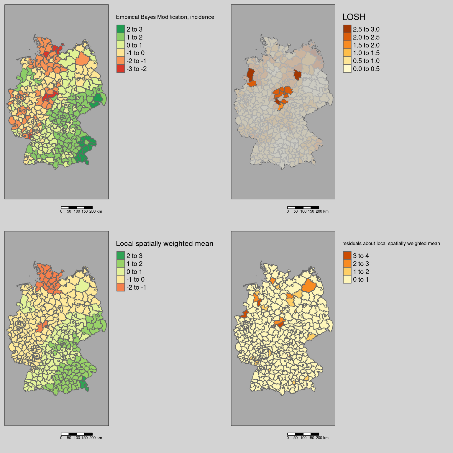
The see that were are two larger blocks of district with large heteroscedasticity:
- one around Göttingen, Kassel and the neighboring districts in Thuringia. which seem to indicate differences between districts in Lower Saxony and Thuringia
- the other covering the Rheine/Ibbenbüren and the Emsland which were characterized by higher incidence rates compared to the districts of the Ruhrgebiet, Osnabrück, Bremen and the districts further up north
In addition, the neighborhood of Stendal is flagged as an area of high spatial heterogeneity.
9.4 German administrative statistics
To show the diversity of local patterns we apply the local indicators on a few other attributes. All examples use the INKAR administrative statistics at the level of the german districts
9.4.1 Share of votes for right-winged party
covidKreise$localM_afd <- getLocalMoranFactor(covidKreise$Stimmenanteile.AfD, listw = unionedListw_d, pval=0.05)m1 <- tm_shape(covidKreise) +
tm_polygons(fill="localM_afd",
fill.scale= tm_scale_categorical(values= localMcPalette),
fill.legend= tm_legend(title = "Local Moran's I",
reverse=TRUE)
) +
tm_layout(legend.outside = TRUE, bg.color = "darkgrey", outer.bg.color = "lightgrey",
legend.outside.size = 0.5, attr.outside = TRUE,
legend.outside.position = "right") +
tm_scalebar(position = tm_pos_out()) +
tm_title("LISA of votes")
m2 <- tm_shape(covidKreise) +
tm_polygons(fill="Stimmenanteile.AfD",
fill.scale= tm_scale_intervals(values= "-plasma"),
fill.legend= tm_legend(title = "Share votes right winged",
reverse=TRUE)
) +
tm_layout(legend.outside = TRUE, bg.color = "darkgrey", outer.bg.color = "lightgrey",
legend.outside.size = 0.5, attr.outside = TRUE,
legend.outside.position = "left") +
tm_scalebar(position = tm_pos_out()) +
tm_title("Votes")
tmap_arrange(m1, m2)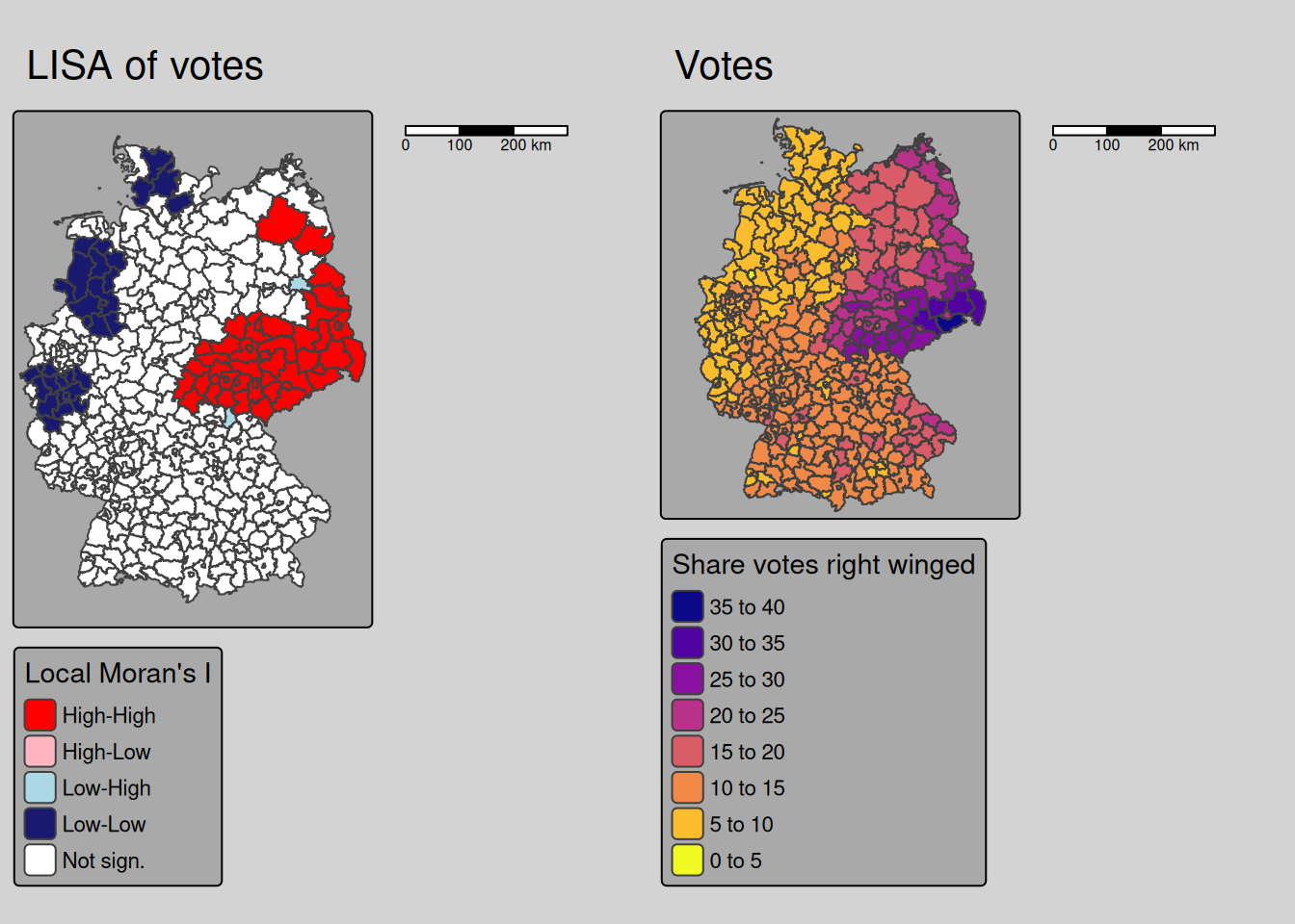
Moran’s I highlights the big spatial cluster of high votes for the AFD in parts of the eastern part of Germany as well as two low outliers attached to the cluster (Berlin and Kronach). It further indicates three spatial clusters of districts with low votes for the AFD in the North and the West (around Cologne-Bonn and around Münster-Osnabrück).
##         GEN
## 278 Kronach
## 326 Berlin## [1] "Neumünster" "Dithmarschen"
## [3] "Rendsburg-Eckernförde" "Schleswig-Flensburg"
## [5] "Segeberg" "Osnabrück"
## [7] "Ammerland" "Cloppenburg"
## [9] "Emsland" "Grafschaft Bentheim"
## [11] "Leer" "Oldenburg"
## [13] "Osnabrück" "Vechta"
## [15] "Mönchengladbach" "Rhein-Kreis Neuss"
## [17] "Bonn" "Köln"
## [19] "Leverkusen" "Düren"
## [21] "Rhein-Erft-Kreis" "Euskirchen"
## [23] "Heinsberg" "Oberbergischer Kreis"
## [25] "Rheinisch-Bergischer Kreis" "Rhein-Sieg-Kreis"
## [27] "Münster" "Steinfurt"
## [29] "Warendorf" "Gütersloh"
## [31] "Ahrweiler" "Neuwied"
## [33] "Vulkaneifel"9.4.2 Long term unemployment rate
covidKreise$localM_lunempl <- getLocalMoranFactor(covidKreise$Langzeitarbeitslosenquote, listw = unionedListw_d, pval=0.05)m1 <- tm_shape(covidKreise) +
tm_polygons(fill="localM_lunempl",
fill.scale= tm_scale_categorical(values= localMcPalette),
fill.legend= tm_legend(title = "Local Moran's I",
reverse=TRUE)
) +
tm_layout(legend.outside = TRUE, bg.color = "darkgrey", outer.bg.color = "lightgrey",
legend.outside.size = 0.5, attr.outside = TRUE,
legend.outside.position = "right") +
tm_scalebar(position = tm_pos_out()) +
tm_title("LISA for long term unemployment")
m2 <- tm_shape(covidKreise) +
tm_polygons(fill="Langzeitarbeitslosenquote",
fill.scale= tm_scale_intervals(values= "-plasma"),
fill.legend= tm_legend(title = "Unemployment rate",
reverse=TRUE)
) +
tm_layout(legend.outside = TRUE, bg.color = "darkgrey", outer.bg.color = "lightgrey",
legend.outside.size = 0.5, attr.outside = TRUE,
legend.outside.position = "right") +
tm_scalebar(position = tm_pos_out()) +
tm_title("Long term unemployment")
tmap_arrange(m1, m2)## [plot mode] fit legend/component: Some legend items or map compoments do not
## fit well, and are therefore rescaled.
## ℹ Set the tmap option `component.autoscale = FALSE` to disable rescaling.
## [plot mode] fit legend/component: Some legend items or map compoments do not
## fit well, and are therefore rescaled.
## ℹ Set the tmap option `component.autoscale = FALSE` to disable rescaling.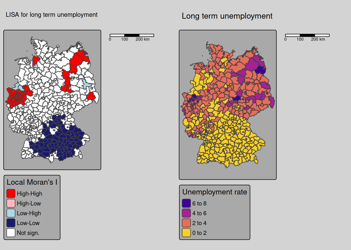
Local Moran’s I indicates a cluster of low longterm unemployment rates in Bavaria and Baden-Württemberg as well as clusters of high values at the Ruhr-Gebiet and some eastern districts as well as Cuxhaven at the North. Schweinsfurt is a high outlier in the southern cluster of low long term unemployment rates.
##  [1] "Cuxhaven"                    "Düsseldorf"
##  [3] "Duisburg"                    "Essen"
##  [5] "Krefeld"                     "Mönchengladbach"
##  [7] "Mülheim an der Ruhr"         "Oberhausen"
##  [9] "Remscheid"                   "Solingen"
## [11] "Wuppertal"                   "Kleve"
## [13] "Mettmann"                    "Rhein-Kreis Neuss"
## [15] "Viersen"                     "Wesel"
## [17] "Köln"                        "Leverkusen"
## [19] "Düren"                       "Rhein-Erft-Kreis"
## [21] "Heinsberg"                   "Oberbergischer Kreis"
## [23] "Rheinisch-Bergischer Kreis"  "Bottrop"
## [25] "Gelsenkirchen"               "Münster"
## [27] "Recklinghausen"              "Warendorf"
## [29] "Bochum"                      "Dortmund"
## [31] "Hagen"                       "Hamm"
## [33] "Herne"                       "Ennepe-Ruhr-Kreis"
## [35] "Märkischer Kreis"            "Soest"
## [37] "Unna"                        "Ostprignitz-Ruppin"
## [39] "Mecklenburgische Seenplatte" "Vorpommern-Greifswald"
## [41] "Bautzen"                     "Anhalt-Bitterfeld"
## [43] "Jerichower Land"             "Salzlandkreis"
## [45] "Stendal"## [1] "Schweinfurt"## [1] "Osterholz" "Friesland" "Borken" "Coesfeld"
## [5] "Dahme-Spreewald"References
We show an approach based on the bootstrap based on the code availabel at https://stackoverflow.com/questions/45177590/map-of-bivariate-spatial-correlation-in-r-bivariate-lisa↩︎