Chapter 13 Spatial regression: spatial lag, spatial error and spatial lagged predictor models
## Loading required package: sf## Linking to GEOS 3.12.1, GDAL 3.8.4, PROJ 9.4.0; sf_use_s2() is TRUE## Loading required package: spdep## Loading required package: spData## To access larger datasets in this package, install the spDataLarge
## package with: `install.packages('spDataLarge',
## repos='https://nowosad.github.io/drat/', type='source')`## Loading required package: ggpubr## Loading required package: ggplot2## Loading required package: spatialreg## Loading required package: Matrix##
## Attaching package: 'spatialreg'## The following objects are masked from 'package:spdep':
##
## get.ClusterOption, get.coresOption, get.mcOption,
## get.VerboseOption, get.ZeroPolicyOption, set.ClusterOption,
## set.coresOption, set.mcOption, set.VerboseOption,
## set.ZeroPolicyOption## Loading required package: tidyverse## ── Attaching core tidyverse packages ──────────────────────── tidyverse 2.0.0 ──
## ✔ dplyr 1.1.4 ✔ readr 2.1.5
## ✔ forcats 1.0.0 ✔ stringr 1.5.1
## ✔ lubridate 1.9.3 ✔ tibble 3.2.1
## ✔ purrr 1.0.2 ✔ tidyr 1.3.1
## ── Conflicts ────────────────────────────────────────── tidyverse_conflicts() ──
## ✖ tidyr::expand() masks Matrix::expand()
## ✖ dplyr::filter() masks stats::filter()
## ✖ dplyr::lag() masks stats::lag()
## ✖ tidyr::pack() masks Matrix::pack()
## ✖ tidyr::unpack() masks Matrix::unpack()
## ℹ Use the conflicted package (<http://conflicted.r-lib.org/>) to force all conflicts to become errors## Loading required package: tmap## Loading required package: GGally
## Registered S3 method overwritten by 'GGally':
## method from
## +.gg ggplot213.1 Cheat sheet
The functions are all available in the spatialreg package.
spautolm- maximum likelihood estimation of spatial conditional and simultaneous autoregression modelslagsarlm- maximum likelihood estimation of spatial simultaneous autoregressive lag and spatial Durbin models
13.2 Theory
With the exception of the spatial lagged predictor model which is suitable for most types of regression models (including GLM, GAM, random forest, boosted regression models) the spatial lag and error models described here are only suitable for linear models - i.e. assuming a gaussian distributed error term.
All the models incorporate spatial dependencies based on the spatial weight matrix W:
- the spatial lagged predictor model (SLX) includes lagged predictors
- the spatial error model (SEM) includes a spatially correlated error term
- the spatial lag model (SLM) includes the spatially lagged response variable as an predictor
- the spatial Durban model includes both the spatially lagged response variable as a predictor and a spatially lagged error term
- SEM + SLM
- the Cliff-Ord spatial model includes in addition to the spatial Durban model also a lagged predictor term
- SEM + SLM + SLX
Further details about the approaches can e.g. be found in Anselin and Rey (2014), Haining and Li (2020), Fortin and Dale (2005) or Bivand et al. (2021).
13.2.1 Spatial lagged predictor model (SLX)
\[ y = X\beta + W X \gamma + \epsilon\] There \(W X \gamma\) is representing the spatially lagged predictors for which regression coefficients \(\gamma\) are estimated, in addition to the “normal” predictor variables \(X\) for which regression coefficients \(\beta\) are estimated.
The lagged predictors are nothing more than the weighted mean of the predictor variables of the neighboring spatial units (if \(W\) is row-standardized). Model selection can lead to different sets of lagged and non-lagged predictor variables in the model. Collinearity between lagged and non-lagged predictor variables can be a problem that is encoutered in practice.
13.2.2 Spatial error model
\[\begin{equation} y = X\beta + u \tag{13.1} \end{equation}\]
\[\begin{equation} u = \lambda W u + \epsilon \tag{13.2} \end{equation}\]
where \(y\) is an (N × 1) vector of observations on a dependent variable taken at each of N locations, \(X\) is an (N × k) matrix of exogenous variables, \(\beta\) is an (k × 1) vector of parameters, \(\epsilon\) is an (N × 1) vector of disturbances (uncorrelated errors, typically normally distributed and centered at around zero, however heteroscedasticity is allowed) and \(\lambda\) is a scalar spatial error parameter, and \(u\) is a spatially autocorrelated disturbance vector with constant variance and covariance terms specified by a fixed (N × N ) spatial weights matrix \(W\) and a single coefficient \(\lambda\).
The equation (13.2) can be rearranged to the reduced from:
\[\begin{equation} u = (I - \lambda W)^{-1} \tag{13.3} \end{equation}\]
Substituting equation (13.3) in equation (13.1) leads to:
\[\begin{equation} y = X\beta + (I - \lambda W)^{-1} \epsilon \tag{13.4} \end{equation}\]
Which can be further rearranged to
\[\begin{equation} (I - \lambda W) y = (I - \lambda W) X\beta + \epsilon \tag{13.5} \end{equation}\]
This implies that by both sides of the equation with the spatial filter \((I - \lambda W)\) removes the spatial autocorrelation from the error term on the right hand side of the equation. If heteroscedasticity is present in the error term, this would not be removed by this step. The application of the spatial filter is called a spatial Cochrane-Orcutt transformation.
If we knew the value of the spatial autoregressive parameter \(\lambda\), equation (13.5) would simplify to a linear regression of the spatially filtered response \(y_s = y - \lambda Wy\) and the spatially filtered predictors \(X_s = X - \lambda WX\):
\[\begin{equation} y_s = X_s\beta + \epsilon \tag{13.6} \end{equation}\]
In that sense we can treat \(\lambda\) as a nuisance parameter. Nicely, the precision of the estimate of \(\lambda\) does not effect the precision of the estimate of \(\beta\), as long as the predictors are not correlated with the error term as it is the case for endogenous predictor variables (Anselin and Rey, 2014, p. 201).
The variance-covariance matrix of the errors \(u\) takes the form:
\[ E[uu^T] = (I -\lambda W)^{-1} \Theta (I -\lambda W^T)^{-1}\] \(\Theta\) is the variance-covariance matrix of the uncorrelated error term. If the error term is homoscedastic (\(E[\epsilon_i^2] = \sigma^2\))then the equation simplifies to:
\[ E[uu^T] = \sigma^2((I -\lambda W) (I -\lambda W^T))^{-1}\]
If \(W\) is not symmetric, then \(W \neq W^T\)
13.2.3 Spatial lag model or simultaneous autoregressive model (SAR)
If we the value of the response of one spatial unit depends on the value of its neighbors, this leads to dependencies between all spatial units - at least for those that have neighbors. The response value of district \(i\) depends on the values of its neighbors, say \(j\) and \(k\). If \(i\) is considered a neighbor of \(j\) as well, this implies that \(y_i\) depends on \(y_k\) and that \(y_k\) depends on \(y_i\). Therefore, a system of equations has to be solved simultaneously. That is there the name \(simultaneous\) comes from.
\[ y = X\beta + \rho W y + \epsilon\]
13.2.3.1 Coefficient interpretation and the spatial multiplier
If a spatial lag component (relationship of the response on a lagged version of the response) is part of the model, feedbacks between the spatial units needs to be considered then interpreting the marginal effects. Without that feedback, the marginal effect of the model is specified by the regression coefficients \(\beta\). The feedback effects become clearer if we rearrange the equation:
\[\begin{align} y - \rho W y & = & X \beta + \epsilon \\ (I - \rho W) y & = & X \beta + \epsilon \\ y & = & (I - \rho W)^{-1} x \beta + (I - \rho W)^{-1}\epsilon \end{align}\]
where \(I\) is the n × n identity matrix. This means that the expected impact of a unit change in an exogenous variable \(r\) for a single observation \(i\) on the dependent variable \(y_i\) is no longer equal to \(\beta_r\) , unless \(\rho = 0\). The awkward n × n \(S_r (W) = ((I − \rho W)^{−1} I \beta_r )\) matrix term is needed to calculate impact measures for the spatial lag model, and its generalization, then \(\rho \neq 0\) (Bivand et al., 2021).
Interpretation can be simplified, if we assume a similar unit change to all spatial units for the predictor \(r\) (Anselin and Rey, 2014). The total effect is then \(\frac{\beta_r}{1-\rho}\). The total effect consists of the direct effect, expressed by \(\beta_r\) and the indirect effect by the spatial interaction \(\beta_r \frac{\rho}{1-\rho}\). As \(|\rho| < 1\) the spatial multiplier effect amplifies the direct effect of \(x_r\) at each location. The indirect effect involves thereby not only the neighbors of first order but also higher term neighbors. As \(|\rho| < 1\) this distance decay effect tends to die out relatively soon, i.e. in practice observations far enough (in terms of the neighborhood definition used) from each other will only show a negligible spatial correlation between them.
Formally, the change of the predictor value of one spatial unit can be expressed by a Taylor series approximation:
\[ \Delta y = (\Delta x_r) \beta_r + \rho W (\Delta x_r) \beta_r + \rho^2 W^2 (\Delta x_r) \beta_r + \rho^3 W^3 (\Delta x_r) \beta_r + ... \] \(W^n\) thereby expresses the n-th order neighbors.
13.2.4 Spatial Durban model
\[ y = X\beta + W X \gamma + \rho W y + \epsilon\] there $W X $ is representing the spatially lagged predictors for which regression coefficients \(\gamma\) are estimated
13.2.5 Spatial autoregressive model with autoregressive error term (SARAR)
\[ y = X\beta + W X \gamma + u \] \[ u = \lambda W u + \epsilon \]
13.2.6 SARAR model with lagged response
\[ y = X\beta + W X \gamma + \rho W y + u \]
\[ u = \lambda W u + \epsilon \] The combination of spatial lag and error in a model complicates parameter estimation. Therefore, we often try to avoid this type of model
13.2.7 Test
13.2.7.1 Lagrange multiplier or Rao’s score tests
Moran’s I for regression residuals provides no guidance in choosing between spatial error and spatial lag models. Lagrange multiplier (LM) or Rao’s score tests can be used for that purpose Anselin (1988). 7 These are five tests (Bivand et al., 2021):
- a test for residual autocorrelation (
RSerr) which tests the null hypothesis \(\lambda = 0\) - with a robust version (
adjRSerr) for error dependence in the presence of spatial dependence in the response RSlagfor an omitted spatially lagged response, which tests the null hypothesis \(\rho = 0\)- with
adjRSlagrobust to the simultaneous presence of residual dependence - the portmanteau test
SARMAwhich is the sum ofRSerrandadjRSlag:RSerr + adjRSlag.
The tests should be performed in a specific order. First, RSerr and RSlag should be performed to test if \(\lambda = 0\) or \(\rho = 0\). If one of those is significant and the other not, one should use the lag or the error model. The problem is, that presence of a spatial lag effect can be misinterpreted as a spatial error effect and vice versa. In other words, the RSerr test might be significant due to the presence of the spatial lag effect and RSlag might be significant due to the presence of a spatial error effect. Therefor, if both RSerr and RSlag are significant, then one should use the robust test to check which model structure should be used. One should never use the robust test if only one of RSerr or RSlag was significant and the other not. If only one of adjRSerr and adjRSlag is significant than the spatial lag model (if adjRSlag is significant) or the spatial error model should be used. If again, both tests are significant, one could go for the model structure which had a higher significance value. If both are to close to call, then one might try both models and compare them by a likelihood ratio test. It might also be worth to check in such cases, if the structural part of the model can be improved. If the fit of the model is not good enough, this often leads to situations there both adjRSerr and adjRSlag are significant. The portmanteau test is tricky as it reports the sum of both the lag and the error effect.
The Lagrange multiplier test are score tests, which assess constraints on statistical parameters based on the gradient of the likelihood function (the score), evaluated at the hypothesized parameter value under the null hypothesis. If the restricted estimator is near the maximum likelihood it should not differ from zero by more than the sampling error. While the finite sample distribution of score tests are not known, the follow asymptotically a \(\chi^2\) distribution. Score tests are less specific than the Likelihood-Ratio test or the Wald test. However they only require the computation of the restricted estimator. This makes it feasible to test even when the unconstrained maximum likelihood estimate is a boundary point in the parameter space (such as \(\lambda = 0\) or \(\rho = 0\)).
RSlag tests the null hypothesis
\[H_0: \rho = 0\]
for the regression model that includes a spatially lagged response variable:
\[ y = \rho W y + X \beta + \epsilon \] The alternative hypothesis is:
\[H_1: \rho \neq 0 \]
The test for this case can be expressed as follows:
\[ LM_{\rho} = \frac{d^2_{\rho}}{D} \sim \chi^2(1)\] \(\sim \chi^2(1)\) implies that the test statistic is asymptotically following a \(\chi^2\) distribution with one degree of freedom.
\[d_{\lambda} = \frac{e^TWy}{\hat{\sigma}^2_{ML}}\]
with \(e\) as the OLS residuals, \(Wy\) the spatial lag term and \(\hat{\sigma}^2_{ML} = \frac{e^Te}{n}\).
The denominator \(D\) consists of two parts: i) the sum of the residuals in a regression of the spatially lagged predicted values \(WX\hat{\beta}\) on \(X\) and, ii) a trace expression (\(T = tr(WW+W^TW)\)):
\[ D = \frac{ WX\hat{\beta}^T (I-X(X^TX)^{-1}X^T)WX\hat{\beta}}{\hat{\sigma}^2_{ML}} + tr(WW+W^TW)\] The trace of a square matrix is the sum of its diagonal elements which is equivalent to the sum of the eigenvalues of the matrix.
For RSerr the alternative (so called focused alternative) is a linear regression model that includes a spatial autoregressive or a spatially moving error term:
\[ u = \lambda W u +\epsilon \]
for the spatial autoregressive form, and
\[ u = \lambda W \epsilon + \epsilon \]
for the spatially moving error term. The test cannot distinguish between the two cases which are considered locally equivalent alternatives.
The null hypothesis in both cases is: \[ H_0 : \rho = 0 \]
and the alternative hypothesis:
\[ H_1: \lambda \neq 0 \].
The test for this case can be expressed as follows:
\[ LM_{\lambda} = \frac{d^2_{\rho}}{T} \sim \chi^2(1)\]
\[d_{\lambda} = \frac{e^TWe}{\hat{\sigma}^2_{ML}} \]
The denominater in the test statistic is the same matrix trace \(T\) as above: \(T = tr(WW+W^TW)\).
As the test have also power against the alternative form (lag versus error model), a robust form was developed. In essence, that statistic corrects the original statistic for the potential effect of the “other” alternative, by subtracting a value. The value is the covariance between \(d_\rho\) and \(d_\lambda\). This means that the robustified statistic will always be smaller than the original statistic. If the alternative considered was the correct one, the correction would be minimal and the test statistic would still be significant. If the alternative considered would not be correct, however, the correction would be big and the test statistic will no longer be significant.
For the spatial lag test the robustified test statistics is:
\[ LM_\rho^* = \frac{(d_\rho - d_\lambda)^2}{D-T} \sim \chi^2(1) \] For the spatial error test the robustified test statistics is:
\[ LM_\lambda^* = \frac{(d_\lambda - TD^{-1} d_\rho)^2}{T(1-TD)} \sim \chi^2(1) \] For spatial regression model, a joint test can be developed based on the following test statistics:
\[LM_{\rho \lambda} = LM_\lambda + LM_\rho^*\] \[LM_{\lambda \rho} = LM_\rho + LM_\lambda^*\] Both test statistics are \(\chi^2(2)\) distributed.
13.2.7.2 Spatial Hausmann Test
If the underlying process is truly a spatial error process and the predictors are not correlated with the error term, then both OLS and the spatial lag model should lead to consistent estimates, only the standard error should differ. This consistency is tested by the spatial Hausmann Test (Kelley Pace and LeSage, 2008). The spatial Hausman test tests the null hypothesis that SEM and OLS are two consistent estimators differing in efficiency, and under the alternative hypothesis of misspecification the two estimators yield divergent results.
13.2.8 Comparision to spatial eigenvector mapping
The spatial lag and error model approaches use all eigenvectors of the spatial weight matrix \(W\) while the spatial eigenvector approach uses only those that have an association with the response. Therefore, we can consider the spatial eigenvector approach more precise.
Another advantage of the spatial eigenvector mapping approach is that it works with GLMs and not just normally distributed error terms. There are approaches that transfer the spatial lag approach to poisson and binomial distributed data - however, the approach is limited to negative spatial autocorrelation.
An advantage of the spatial lag model is that it models truly autocorrelated processes and is not limited to induced autocorrelation.
13.3 Case studies
13.3.1 Boston housing data
The Boston housing dataset contains a classical dataset (Harrison and Rubinfeld, 1978) which has been corrected (Gilley and Pace, 1996). The hypothesis investigated is that air pollution influences housing prices which is used to estimate the willingness to pay. Median housing prices for single family houses are available at the level of 506 census tracts in Boston and neighboring town. Airpollution originates from a simulation model that was parameterized by local measurements. The model prediction was available for 98 model units and has been probably assigned to the census tracts that overlap with the modelling units (assignment by largest area if partial overlap). As housing prices depend on other factors (hedonic price model) these have been recorded as well. Some of those variables were available at census tract level while others have only been available at the level of the town and seem to have been copied to the census tracts they overlap.
The following columns are present in the sf object:
TOWNa factor with levels given by town namesTOWNNOa numeric vector corresponding to TOWNTRACTtract ID numbersLONtract point longitudes in decimal degreesLATtract point latitudes in decimal degreesMEDVmedian values of owner-occupied housing in USD 1000CMEDVcorrected median values of owner-occupied housing in USD 1000CRIMper capita crime; presumably negative effect on housing priceZNproportions of residential land zoned for lots over 25000 sq. ft per town (constant for all Boston tracts). Since such zoning restricts construction of small lot houses, it might be positively related to housing values. A positive coefficient may also arise because zoning proxies the exclusivity, social class, and outdoor amenities of a community.INDUSproportions of non-retail business acres per town (constant for all Boston tracts); serves as a proxy for the externalities associated with industry-noise, heavy traffic, and unpleasant visual effects, and thus should affect housing values negatively.CHASa factor with levels 1 if tract borders Charles River; 0 otherwise. Presuambly positively associated with housing price.NOXnitric oxides concentration (parts per 10 million) per town. This is the main predictor, the original analysis was intereset in. The rest are more confounding factors to be controllted for.RMaverage numbers of rooms per dwelling, should be positively associated with housing valueAGEproportions of owner-occupied units built prior to 1940; unit age is assumed to be related to structure quality. Higher share of old units is therefore hypothesized to be associated with lower housing value.DISweighted distances to five Boston employment centersRADindex of accessibility to radial highways per town (constant for all Boston tracts)TAXfull-value property-tax rate per USD 10,000 per town (constant for all Boston tracts). Should be negatively associated with housing value.PTRATIOa numeric vector of pupil-teacher ratios per town (constant for all Boston tracts)B1000*(Bk - 0.63)^2 where Bk is the proportion of blacks. At low to moderate levels of B, an increase should have a negative influence on housing value if Blacks are regarded as undesirable neighbors by Whites. However, market discrimination means that housing values are higher at very high levels of R. One expects, therefore, a parabolic relationship between proportion Black in a neighborhood and housing values.LSTATpercentage values of lower status population (proportion of adults without some high school education and proportion of male workers classified as workers).unitsnumber of single family housescu5kcount of units under USD 5,000c5_7_5counts USD 5,000 to 7,500C_interval countsco50kcount of units over USD 50,000medianrecomputed median valuesBBrecomputed black population proportioncensoredwhether censored or notNOXIDNOX model zone IDPOPtract population
## Reading layer `boston' from data source
##   `/home/slautenbach/Documents/lehre/HD/git_areas/spatial_data_science/spatial-data-science/data/boston.gpkg'
##   using driver `GPKG'
## Simple feature collection with 506 features and 36 fields
## Geometry type: POLYGON
## Dimension:     XY
## Bounding box:  xmin: 291912.3 ymin: 4651542 xmax: 364541.7 ymax: 4726401
## Projected CRS: WGS 84 / UTM zone 19N## poltract TOWN TOWNNO TRACT
## Length:506 Length:506 Min. : 0.00 Min. : 1
## Class :character Class :character 1st Qu.:26.25 1st Qu.:1303
## Mode :character Mode :character Median :42.00 Median :3394
## Mean :47.53 Mean :2700
## 3rd Qu.:78.00 3rd Qu.:3740
## Max. :91.00 Max. :5082
##
## LON LAT MEDV CMEDV
## Min. :-71.29 Min. :42.03 Min. : 5.00 Min. : 5.00
## 1st Qu.:-71.09 1st Qu.:42.18 1st Qu.:17.02 1st Qu.:17.02
## Median :-71.05 Median :42.22 Median :21.20 Median :21.20
## Mean :-71.06 Mean :42.22 Mean :22.53 Mean :22.53
## 3rd Qu.:-71.02 3rd Qu.:42.25 3rd Qu.:25.00 3rd Qu.:25.00
## Max. :-70.81 Max. :42.38 Max. :50.00 Max. :50.00
##
## CRIM ZN INDUS CHAS
## Min. : 0.00632 Min. : 0.00 Min. : 0.46 Length:506
## 1st Qu.: 0.08205 1st Qu.: 0.00 1st Qu.: 5.19 Class :character
## Median : 0.25651 Median : 0.00 Median : 9.69 Mode :character
## Mean : 3.61352 Mean : 11.36 Mean :11.14
## 3rd Qu.: 3.67708 3rd Qu.: 12.50 3rd Qu.:18.10
## Max. :88.97620 Max. :100.00 Max. :27.74
##
## NOX RM AGE DIS
## Min. :0.3850 Min. :3.561 Min. : 2.90 Min. : 1.130
## 1st Qu.:0.4490 1st Qu.:5.886 1st Qu.: 45.02 1st Qu.: 2.100
## Median :0.5380 Median :6.208 Median : 77.50 Median : 3.207
## Mean :0.5547 Mean :6.285 Mean : 68.57 Mean : 3.795
## 3rd Qu.:0.6240 3rd Qu.:6.623 3rd Qu.: 94.08 3rd Qu.: 5.188
## Max. :0.8710 Max. :8.780 Max. :100.00 Max. :12.127
##
## RAD TAX PTRATIO B
## Min. : 1.000 Min. :187.0 Min. :12.60 Min. : 0.32
## 1st Qu.: 4.000 1st Qu.:279.0 1st Qu.:17.40 1st Qu.:375.38
## Median : 5.000 Median :330.0 Median :19.05 Median :391.44
## Mean : 9.549 Mean :408.2 Mean :18.46 Mean :356.67
## 3rd Qu.:24.000 3rd Qu.:666.0 3rd Qu.:20.20 3rd Qu.:396.23
## Max. :24.000 Max. :711.0 Max. :22.00 Max. :396.90
##
## LSTAT units cu5k c5_7_5
## Min. : 1.73 Min. : 5.0 Min. : 0.000 Min. : 0.000
## 1st Qu.: 6.95 1st Qu.: 115.0 1st Qu.: 0.000 1st Qu.: 1.000
## Median :11.36 Median : 511.5 Median : 1.000 Median : 3.000
## Mean :12.65 Mean : 680.8 Mean : 2.921 Mean : 5.534
## 3rd Qu.:16.95 3rd Qu.:1152.0 3rd Qu.: 4.000 3rd Qu.: 7.000
## Max. :37.97 Max. :3031.0 Max. :35.000 Max. :70.000
##
## C7_5_10 C10_15 C15_20 C20_25
## Min. : 0.000 Min. : 0.00 Min. : 0.0 Min. : 0.0
## 1st Qu.: 2.000 1st Qu.: 14.00 1st Qu.: 19.0 1st Qu.: 13.0
## Median : 6.000 Median : 33.00 Median : 85.0 Median :101.5
## Mean : 9.984 Mean : 55.41 Mean :141.8 Mean :166.2
## 3rd Qu.: 13.000 3rd Qu.: 75.50 3rd Qu.:210.0 3rd Qu.:281.8
## Max. :121.000 Max. :520.00 Max. :937.0 Max. :723.0
##
## C25_35 C35_50 co50k median
## Min. : 0.0 Min. : 0.00 Min. : 0.00 Min. : 5600
## 1st Qu.: 7.0 1st Qu.: 1.00 1st Qu.: 0.00 1st Qu.:16800
## Median : 95.0 Median : 17.00 Median : 3.00 Median :21000
## Mean : 170.8 Mean : 82.74 Mean : 45.44 Mean :21749
## 3rd Qu.: 292.0 3rd Qu.: 97.00 3rd Qu.: 20.00 3rd Qu.:24700
## Max. :1189.0 Max. :769.00 Max. :980.00 Max. :50000
## NA's :17
## BB censored NOX_ID POP
## Min. : 0.000 Length:506 Min. : 1.00 Min. : 434
## 1st Qu.: 0.200 Class :character 1st Qu.:18.00 1st Qu.: 3697
## Median : 0.500 Mode :character Median :44.00 Median : 5105
## Mean : 6.082 Mean :41.77 Mean : 5340
## 3rd Qu.: 1.600 3rd Qu.:62.00 3rd Qu.: 6825
## Max. :96.400 Max. :96.00 Max. :15976
##
## geom
## POLYGON :506
## epsg:32619 : 0
## +proj=utm ...: 0
##
##
##
## All variables are complete and contain no missing data.
13.3.1.1 Explorative Data Analysis
tm_shape(bostonSf) +
  tm_polygons(col="TOWN", title = "Town name",
               border.alpha = 0.5) +
  tm_scale_bar() +
  tm_layout(main.title = "Town names",
            legend.outside = TRUE, attr.outside = TRUE)
## ## ── tmap v3 code detected ───────────────────────────────────────────────────────## [v3->v4] `tm_polygons()`: use 'fill' for the fill color of polygons/symbols
## (instead of 'col'), and 'col' for the outlines (instead of 'border.col').
## [v3->v4] `tm_polygons()`: use `col_alpha` instead of `border.alpha`.
## [v3->v4] `tm_polygons()`: migrate the argument(s) related to the legend of the
## visual variable `fill` namely 'title' to 'fill.legend = tm_legend(<HERE>)'
## ! `tm_scale_bar()` is deprecated. Please use `tm_scalebar()` instead.
## [v3->v4] `tm_layout()`: use `tm_title()` instead of `tm_layout(main.title = )`
## This message is displayed once every 8 hours.## Warning: Number of levels of the variable assigned to the aesthetic "fill" of
## the layer "polygons" is 92, which is larger than n.max (which is 30), so levels
## are combined.## [plot mode] fit legend/component: Some legend items or map compoments do not
## fit well, and are therefore rescaled.
## ℹ Set the tmap option `component.autoscale = FALSE` to disable rescaling.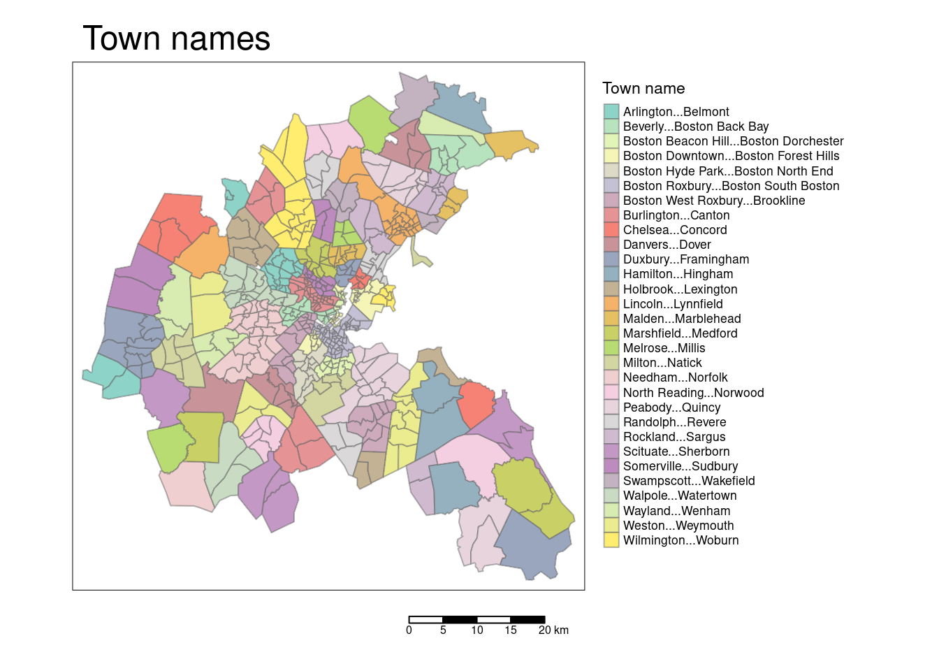
tm_shape(bostonSf) +
  tm_polygons(col="CMEDV", title = "Median value, corrected [USD 1000]",
               border.alpha = 0.5) +
  tm_scale_bar() +
  tm_layout(main.title = "Median values of owner-occupied housing",
            legend.outside = TRUE, attr.outside = TRUE)
## ## ── tmap v3 code detected ───────────────────────────────────────────────────────## [v3->v4] `tm_polygons()`: use `col_alpha` instead of `border.alpha`.
## [v3->v4] `tm_polygons()`: migrate the argument(s) related to the legend of the
## visual variable `fill` namely 'title' to 'fill.legend = tm_legend(<HERE>)'
## ! `tm_scale_bar()` is deprecated. Please use `tm_scalebar()` instead.
## [v3->v4] `tm_layout()`: use `tm_title()` instead of `tm_layout(main.title = )`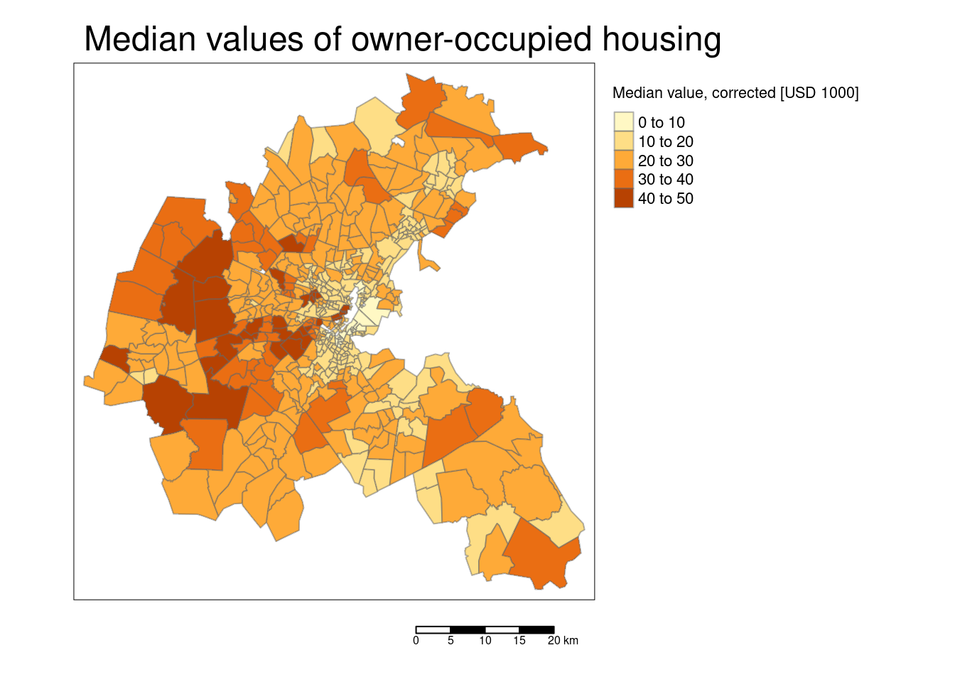
tm_shape(bostonSf) +
tm_polygons(col="NOX", title = "Nitric oxides [pp 10 million]",
border.alpha = 0.5) +
tm_scale_bar() +
tm_layout(main.title = "Nitric oxides concentration",
legend.outside = TRUE, attr.outside = TRUE)## ## ── tmap v3 code detected ───────────────────────────────────────────────────────## [v3->v4] `tm_polygons()`: use `col_alpha` instead of `border.alpha`.
## [v3->v4] `tm_polygons()`: migrate the argument(s) related to the legend of the
## visual variable `fill` namely 'title' to 'fill.legend = tm_legend(<HERE>)'
## ! `tm_scale_bar()` is deprecated. Please use `tm_scalebar()` instead.
## [v3->v4] `tm_layout()`: use `tm_title()` instead of `tm_layout(main.title = )`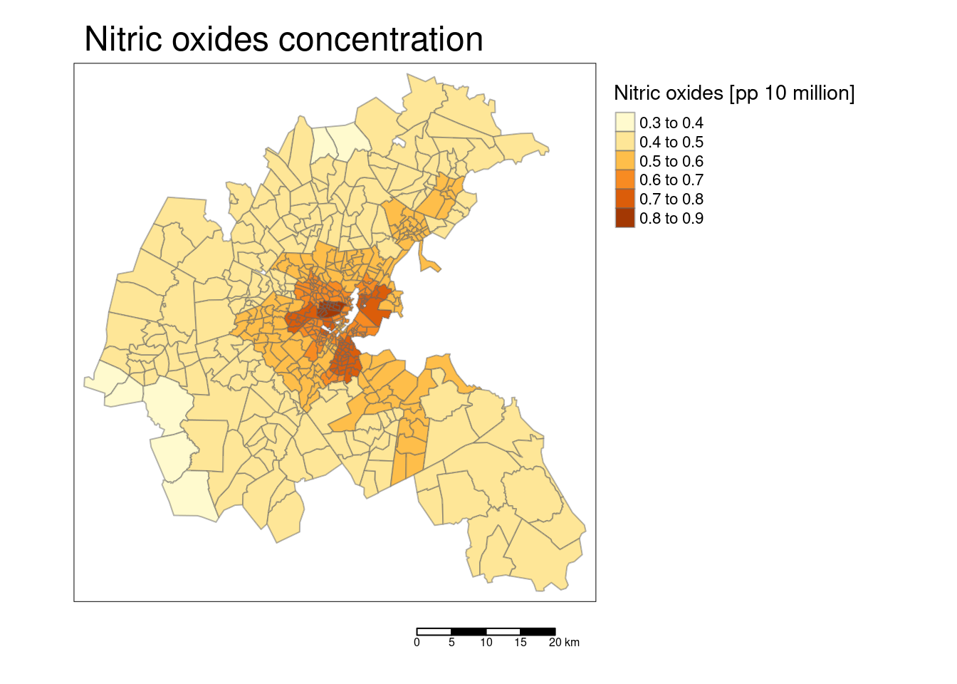
tm_shape(bostonSf) +
tm_polygons(col="CRIM", title = "Crime per capita",
border.alpha = 0.5, style = "kmeans") +
tm_scale_bar() +
tm_layout(main.title = "Crime",
legend.outside = TRUE, attr.outside = TRUE)## ## ── tmap v3 code detected ───────────────────────────────────────────────────────## [v3->v4] `tm_polygons()`: instead of `style = "kmeans"`, use fill.scale =
## `tm_scale_intervals()`.
## ℹ Migrate the argument(s) 'style' to 'tm_scale_intervals(<HERE>)'
## [v3->v4] `tm_polygons()`: use `col_alpha` instead of `border.alpha`.
## [v3->v4] `tm_polygons()`: migrate the argument(s) related to the legend of the
## visual variable `fill` namely 'title' to 'fill.legend = tm_legend(<HERE>)'
## ! `tm_scale_bar()` is deprecated. Please use `tm_scalebar()` instead.
## [v3->v4] `tm_layout()`: use `tm_title()` instead of `tm_layout(main.title = )`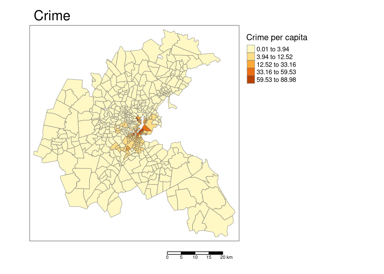
tm_shape(bostonSf) +
tm_polygons(col="RM", title = "Rooms per dwelling",
border.alpha = 0.5, style = "pretty") +
tm_scale_bar() +
tm_layout(main.title = "Average rooms per dwelling",
legend.outside = TRUE, attr.outside = TRUE)## ## ── tmap v3 code detected ───────────────────────────────────────────────────────## [v3->v4] `tm_polygons()`: instead of `style = "pretty"`, use fill.scale =
## `tm_scale_intervals()`.
## ℹ Migrate the argument(s) 'style' to 'tm_scale_intervals(<HERE>)'
## [v3->v4] `tm_polygons()`: use `col_alpha` instead of `border.alpha`.
## [v3->v4] `tm_polygons()`: migrate the argument(s) related to the legend of the
## visual variable `fill` namely 'title' to 'fill.legend = tm_legend(<HERE>)'
## ! `tm_scale_bar()` is deprecated. Please use `tm_scalebar()` instead.
## [v3->v4] `tm_layout()`: use `tm_title()` instead of `tm_layout(main.title = )`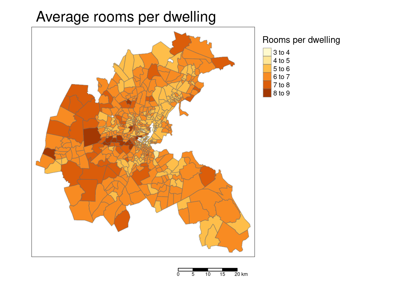
tm_shape(bostonSf) +
  tm_polygons(col="LSTAT", title = "Lower status population [%]",
              border.alpha = 0.5, style = "pretty") +
  tm_scale_bar() +
  tm_layout(main.title = "Lower status population",
            legend.outside = TRUE, attr.outside = TRUE)
## ## ── tmap v3 code detected ───────────────────────────────────────────────────────## [v3->v4] `tm_polygons()`: instead of `style = "pretty"`, use fill.scale =
## `tm_scale_intervals()`.
## ℹ Migrate the argument(s) 'style' to 'tm_scale_intervals(<HERE>)'
## [v3->v4] `tm_polygons()`: use `col_alpha` instead of `border.alpha`.
## [v3->v4] `tm_polygons()`: migrate the argument(s) related to the legend of the
## visual variable `fill` namely 'title' to 'fill.legend = tm_legend(<HERE>)'
## ! `tm_scale_bar()` is deprecated. Please use `tm_scalebar()` instead.
## [v3->v4] `tm_layout()`: use `tm_title()` instead of `tm_layout(main.title = )`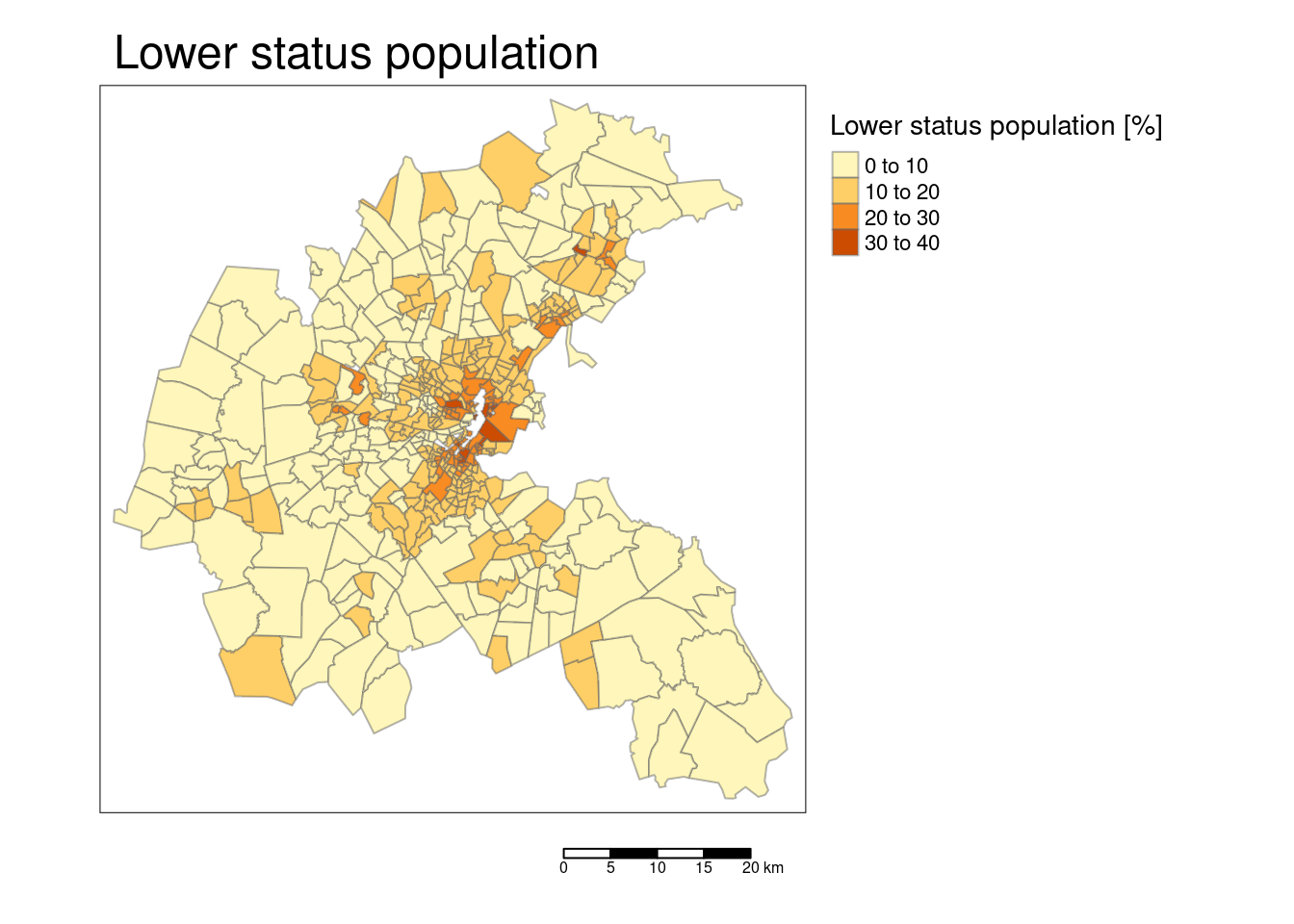
tm_shape(bostonSf) +
  tm_polygons(col="BB", title = "Black population, recomputed [%]",
              border.alpha = 0.5, style = "kmeans") +
  tm_scale_bar() +
  tm_layout(main.title = "Black population",
            legend.outside = TRUE, attr.outside = TRUE)
## ## ── tmap v3 code detected ───────────────────────────────────────────────────────## [v3->v4] `tm_polygons()`: instead of `style = "kmeans"`, use fill.scale =
## `tm_scale_intervals()`.
## ℹ Migrate the argument(s) 'style' to 'tm_scale_intervals(<HERE>)'
## [v3->v4] `tm_polygons()`: use `col_alpha` instead of `border.alpha`.
## [v3->v4] `tm_polygons()`: migrate the argument(s) related to the legend of the
## visual variable `fill` namely 'title' to 'fill.legend = tm_legend(<HERE>)'
## ! `tm_scale_bar()` is deprecated. Please use `tm_scalebar()` instead.
## [v3->v4] `tm_layout()`: use `tm_title()` instead of `tm_layout(main.title = )`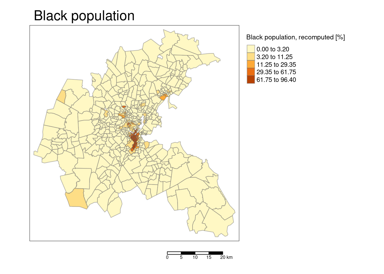
tm_shape(bostonSf) +
  tm_polygons(col="RAD", title = "Accessibility index",
              border.alpha = 0.5, style = "pretty") +
  tm_scale_bar() +
  tm_layout(main.title = "Accessibility to radial highways per town",
            legend.outside = TRUE, attr.outside = TRUE)
## ## ── tmap v3 code detected ───────────────────────────────────────────────────────## [v3->v4] `tm_polygons()`: instead of `style = "pretty"`, use fill.scale =
## `tm_scale_intervals()`.
## ℹ Migrate the argument(s) 'style' to 'tm_scale_intervals(<HERE>)'
## [v3->v4] `tm_polygons()`: use `col_alpha` instead of `border.alpha`.
## [v3->v4] `tm_polygons()`: migrate the argument(s) related to the legend of the
## visual variable `fill` namely 'title' to 'fill.legend = tm_legend(<HERE>)'
## ! `tm_scale_bar()` is deprecated. Please use `tm_scalebar()` instead.
## [v3->v4] `tm_layout()`: use `tm_title()` instead of `tm_layout(main.title = )`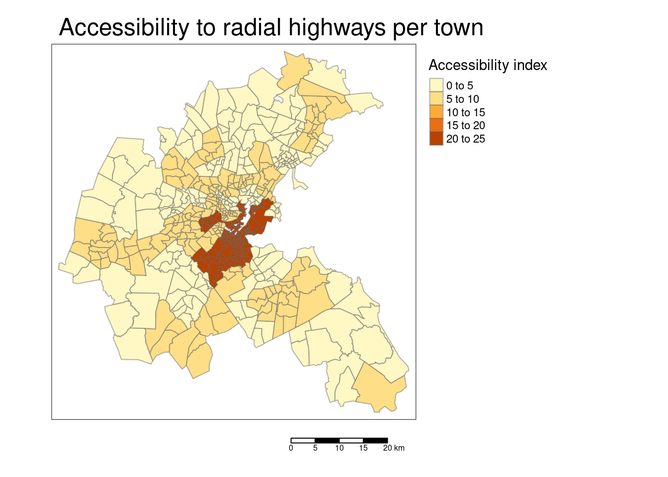
tm_shape(bostonSf) +
  tm_polygons(col="TAX", title = "Property tax rate [per USD 10,000]",
              border.alpha = 0.5, style = "pretty") +
  tm_scale_bar() +
  tm_layout(main.title = "Full-value property-tax rate per town ",
            legend.outside = TRUE, attr.outside = TRUE)
## ## ── tmap v3 code detected ───────────────────────────────────────────────────────## [v3->v4] `tm_polygons()`: instead of `style = "pretty"`, use fill.scale =
## `tm_scale_intervals()`.
## ℹ Migrate the argument(s) 'style' to 'tm_scale_intervals(<HERE>)'
## [v3->v4] `tm_polygons()`: use `col_alpha` instead of `border.alpha`.
## [v3->v4] `tm_polygons()`: migrate the argument(s) related to the legend of the
## visual variable `fill` namely 'title' to 'fill.legend = tm_legend(<HERE>)'
## ! `tm_scale_bar()` is deprecated. Please use `tm_scalebar()` instead.
## [v3->v4] `tm_layout()`: use `tm_title()` instead of `tm_layout(main.title = )`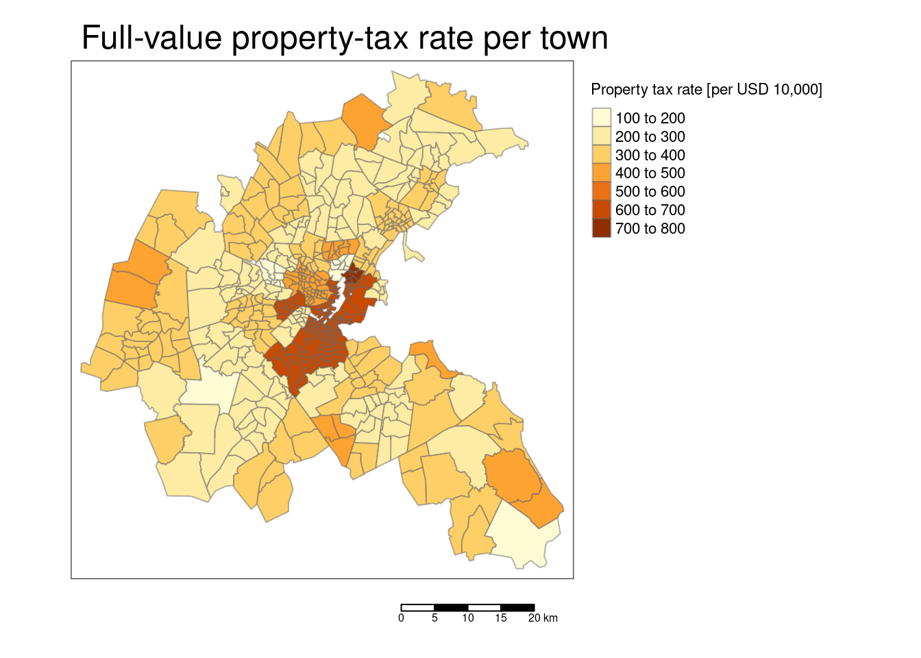
tm_shape(bostonSf) +
  tm_polygons(col="AGE", title = "Owner-occupied units",
              border.alpha = 0.5, style = "pretty") +
  tm_scale_bar() +
  tm_layout(main.title = "Owner-occupied units built prior to 1940 [%]",
            legend.outside = TRUE, attr.outside = TRUE)
## ## ── tmap v3 code detected ───────────────────────────────────────────────────────## [v3->v4] `tm_polygons()`: instead of `style = "pretty"`, use fill.scale =
## `tm_scale_intervals()`.
## ℹ Migrate the argument(s) 'style' to 'tm_scale_intervals(<HERE>)'
## [v3->v4] `tm_polygons()`: use `col_alpha` instead of `border.alpha`.
## [v3->v4] `tm_polygons()`: migrate the argument(s) related to the legend of the
## visual variable `fill` namely 'title' to 'fill.legend = tm_legend(<HERE>)'
## ! `tm_scale_bar()` is deprecated. Please use `tm_scalebar()` instead.
## [v3->v4] `tm_layout()`: use `tm_title()` instead of `tm_layout(main.title = )`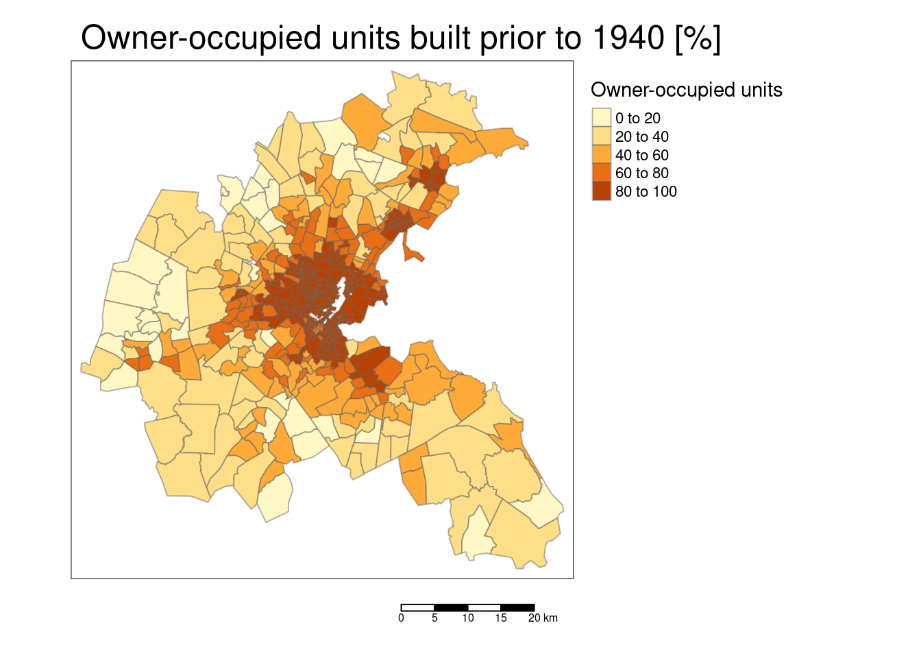
tm_shape(bostonSf) +
  tm_polygons(col="DIS", title = "Distance, weighted",
              border.alpha = 0.5, style = "pretty") +
  tm_scale_bar() +
  tm_layout(main.title = "Distances to five Boston employment centres",
            legend.outside = TRUE, attr.outside = TRUE)
## ## ── tmap v3 code detected ───────────────────────────────────────────────────────## [v3->v4] `tm_polygons()`: instead of `style = "pretty"`, use fill.scale =
## `tm_scale_intervals()`.
## ℹ Migrate the argument(s) 'style' to 'tm_scale_intervals(<HERE>)'
## [v3->v4] `tm_polygons()`: use `col_alpha` instead of `border.alpha`.
## [v3->v4] `tm_polygons()`: migrate the argument(s) related to the legend of the
## visual variable `fill` namely 'title' to 'fill.legend = tm_legend(<HERE>)'
## ! `tm_scale_bar()` is deprecated. Please use `tm_scalebar()` instead.
## [v3->v4] `tm_layout()`: use `tm_title()` instead of `tm_layout(main.title = )`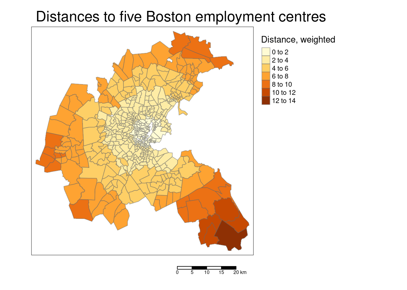
tm_shape(bostonSf) +
  tm_polygons(col="INDUS", title = "Non-retail business acre",
              border.alpha = 0.5, style = "pretty") +
  tm_scale_bar() +
  tm_layout(main.title = "Non-retail business acres per town ",
            legend.outside = TRUE, attr.outside = TRUE)
## ## ── tmap v3 code detected ───────────────────────────────────────────────────────## [v3->v4] `tm_polygons()`: instead of `style = "pretty"`, use fill.scale =
## `tm_scale_intervals()`.
## ℹ Migrate the argument(s) 'style' to 'tm_scale_intervals(<HERE>)'
## [v3->v4] `tm_polygons()`: use `col_alpha` instead of `border.alpha`.
## [v3->v4] `tm_polygons()`: migrate the argument(s) related to the legend of the
## visual variable `fill` namely 'title' to 'fill.legend = tm_legend(<HERE>)'
## ! `tm_scale_bar()` is deprecated. Please use `tm_scalebar()` instead.
## [v3->v4] `tm_layout()`: use `tm_title()` instead of `tm_layout(main.title = )`
tm_shape(bostonSf) +
  tm_polygons(col="CHAS", title = "At river", palette= c("grey", "navy"),
              border.alpha = 0.5, style = "pretty") +
  tm_scale_bar() +
  tm_layout(main.title = "Charles River boundary",
            legend.outside = TRUE, attr.outside = TRUE)
## ## ── tmap v3 code detected ───────────────────────────────────────────────────────## [v3->v4] `tm_polygons()`: instead of `style = "pretty"`, use fill.scale =
## `tm_scale_intervals()`.
## ℹ Migrate the argument(s) 'style', 'palette' (rename to 'values') to
## 'tm_scale_intervals(<HERE>)'
## [v3->v4] `tm_polygons()`: use `col_alpha` instead of `border.alpha`.
## [v3->v4] `tm_polygons()`: migrate the argument(s) related to the legend of the
## visual variable `fill` namely 'title' to 'fill.legend = tm_legend(<HERE>)'
## ! `tm_scale_bar()` is deprecated. Please use `tm_scalebar()` instead.
## [v3->v4] `tm_layout()`: use `tm_title()` instead of `tm_layout(main.title = )`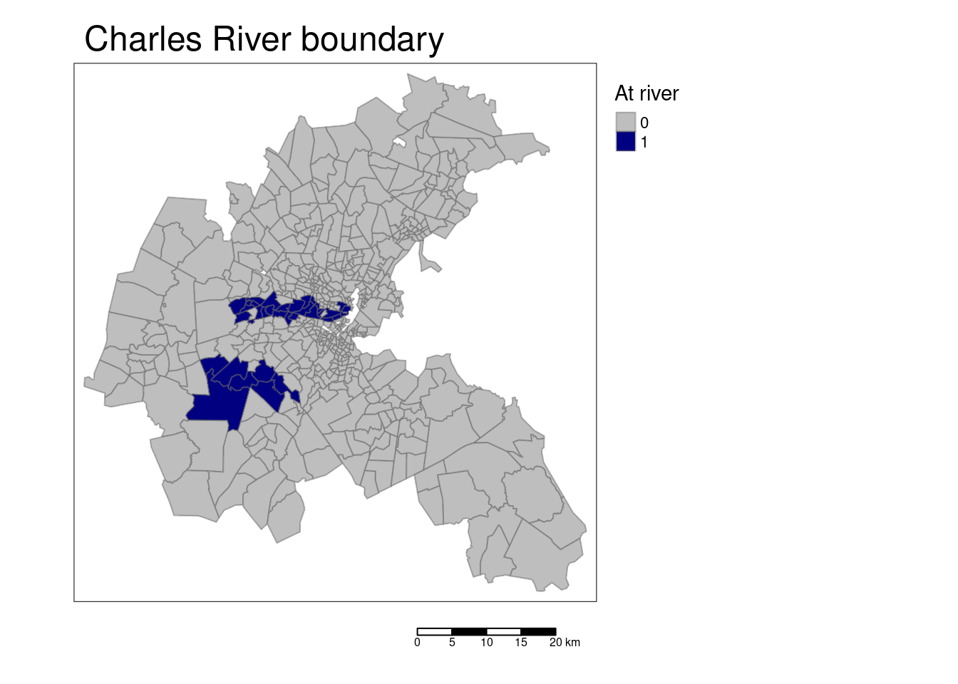
tm_shape(bostonSf) +
  tm_polygons(col="PTRATIO", title = "Pupil-teacher ratio",
              border.alpha = 0.5, style = "pretty") +
  tm_scale_bar() +
  tm_layout(main.title = "Pupil-teacher ratio per town",
            legend.outside = TRUE, attr.outside = TRUE)
## ## ── tmap v3 code detected ───────────────────────────────────────────────────────## [v3->v4] `tm_polygons()`: instead of `style = "pretty"`, use fill.scale =
## `tm_scale_intervals()`.
## ℹ Migrate the argument(s) 'style' to 'tm_scale_intervals(<HERE>)'
## [v3->v4] `tm_polygons()`: use `col_alpha` instead of `border.alpha`.
## [v3->v4] `tm_polygons()`: migrate the argument(s) related to the legend of the
## visual variable `fill` namely 'title' to 'fill.legend = tm_legend(<HERE>)'
## ! `tm_scale_bar()` is deprecated. Please use `tm_scalebar()` instead.
## [v3->v4] `tm_layout()`: use `tm_title()` instead of `tm_layout(main.title = )`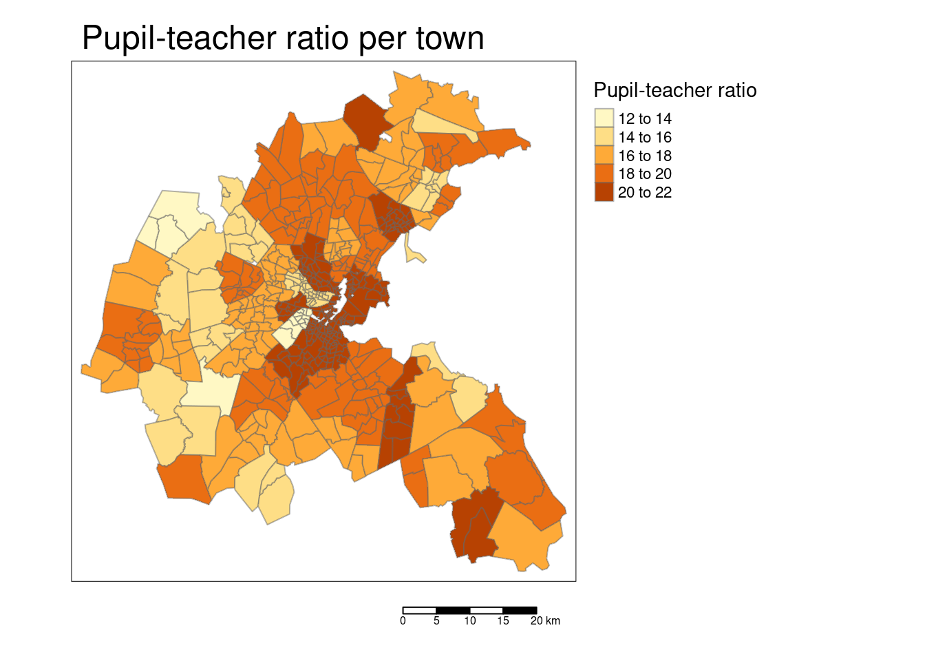
## `stat_bin()` using `bins = 30`. Pick better value with `binwidth`.
## `stat_bin()` using `bins = 30`. Pick better value with `binwidth`.
## `stat_bin()` using `bins = 30`. Pick better value with `binwidth`.
## `stat_bin()` using `bins = 30`. Pick better value with `binwidth`.
## `stat_bin()` using `bins = 30`. Pick better value with `binwidth`.
## `stat_bin()` using `bins = 30`. Pick better value with `binwidth`.
## `stat_bin()` using `bins = 30`. Pick better value with `binwidth`.
## `stat_bin()` using `bins = 30`. Pick better value with `binwidth`.
## `stat_bin()` using `bins = 30`. Pick better value with `binwidth`.
## `stat_bin()` using `bins = 30`. Pick better value with `binwidth`.
## `stat_bin()` using `bins = 30`. Pick better value with `binwidth`.
## `stat_bin()` using `bins = 30`. Pick better value with `binwidth`.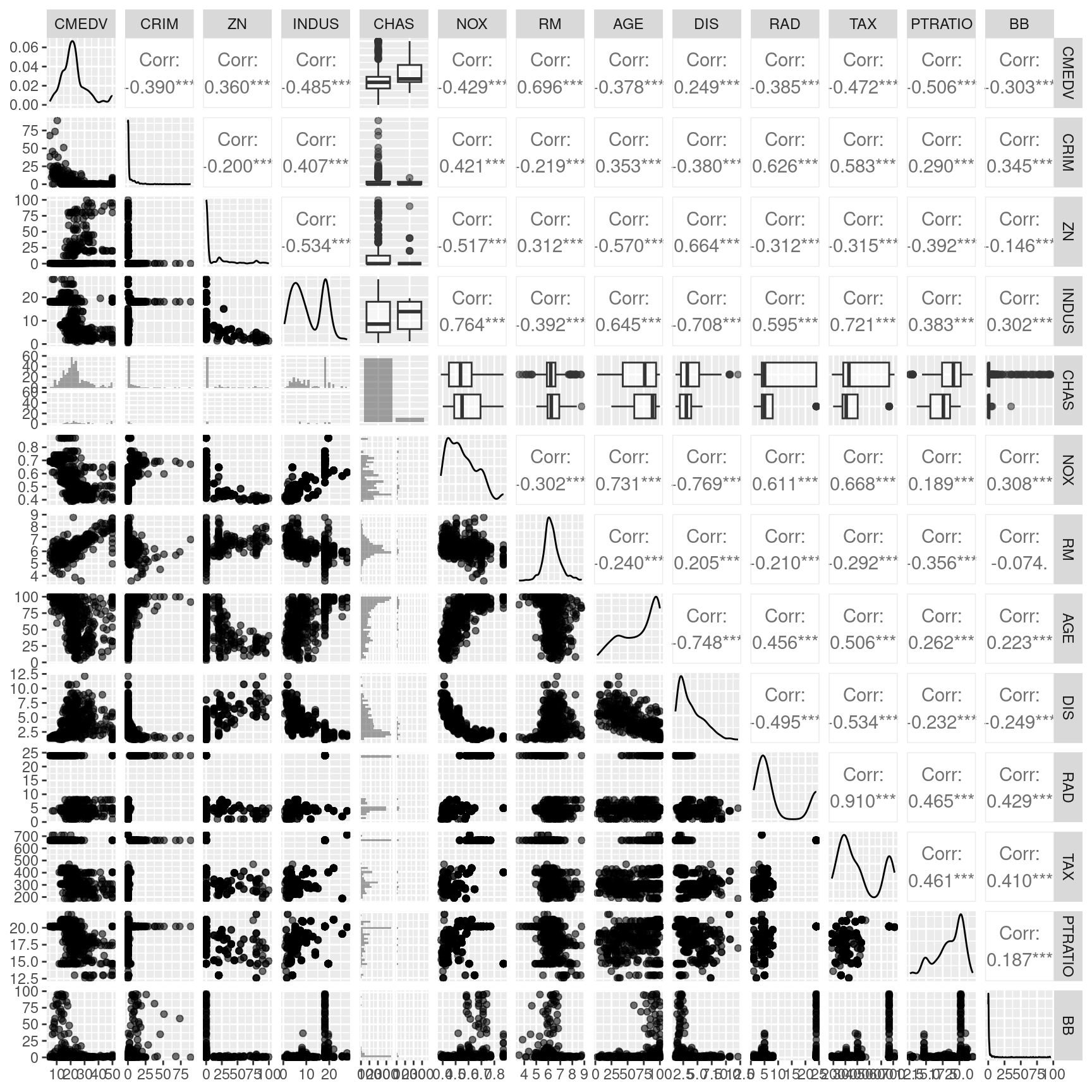
The scatterplot reveals that the response is correlated with all predictors. However, there are also quite some correlations between the different predictors. For example the accessibility to the radial highways and the crime rate are highly correlated, as is crime rate and the full-value property-tax rate. To a lower degree, NOX is as well positively correlated with the crime rate. NOX is also strongly positively correlated with the proportion of owner-occupied units built prior to 1940 and the full-value property-tax rate. NOX is strongly negatively associated with the accessibility to the radial highways. The full-value property-tax rate and the accessibility to radial highways are extremely high positively correlated. The proportion of owner-occupied units built prior to 1940 and the weighted distances to five Boston employment centers are strongly negatively associated. We need to keep this and other correlations in mind then interpreting the results. Even if just one of the collinear predictors is in the final model, the other is implicitly in as well due to the correlation.
13.3.1.2 Linear model
Lets start with a simple linear model, inspired by the literature. poly(,var,n) includes an orthogonal polynomial of order n of the response. In addition, some predictors were log-transformed.
model0 <- lm(CMEDV ~ CRIM + ZN + INDUS + CHAS + poly(NOX,2) + poly(RM,2) +
                    AGE + log(DIS) + log(RAD) + TAX + PTRATIO + poly(BB,2) + log(LSTAT), data = bostonSf)
summary(model0)
##
## Call:
## lm(formula = CMEDV ~ CRIM + ZN + INDUS + CHAS + poly(NOX, 2) +
## poly(RM, 2) + AGE + log(DIS) + log(RAD) + TAX + PTRATIO +
## poly(BB, 2) + log(LSTAT), data = bostonSf)
##
## Residuals:
## Min 1Q Median 3Q Max
## -24.3093 -2.0449 -0.2838 1.7118 24.9687
##
## Coefficients:
## Estimate Std. Error t value Pr(>|t|)
## (Intercept) 60.067833 2.258700 26.594 < 2e-16 ***
## CRIM -0.156348 0.025874 -6.043 3.01e-09 ***
## ZN 0.018154 0.011113 1.634 0.102993
## INDUS -0.001576 0.049170 -0.032 0.974448
## CHAS1 2.256598 0.691785 3.262 0.001184 **
## poly(NOX, 2)1 -44.555978 10.056345 -4.431 1.16e-05 ***
## poly(NOX, 2)2 -8.581016 5.717168 -1.501 0.134021
## poly(RM, 2)1 50.561735 5.568399 9.080 < 2e-16 ***
## poly(RM, 2)2 37.016795 4.130322 8.962 < 2e-16 ***
## AGE -0.002814 0.011482 -0.245 0.806494
## log(DIS) -5.389696 0.763995 -7.055 5.95e-12 ***
## log(RAD) 1.863469 0.401517 4.641 4.46e-06 ***
## TAX -0.008159 0.002545 -3.205 0.001438 **
## PTRATIO -0.647768 0.105714 -6.128 1.84e-09 ***
## poly(BB, 2)1 -14.231271 4.296171 -3.313 0.000993 ***
## poly(BB, 2)2 -0.993125 3.982692 -0.249 0.803187
## log(LSTAT) -7.978762 0.520569 -15.327 < 2e-16 ***
## ---
## Signif. codes: 0 '***' 0.001 '**' 0.01 '*' 0.05 '.' 0.1 ' ' 1
##
## Residual standard error: 3.778 on 489 degrees of freedom
## Multiple R-squared: 0.8361, Adjusted R-squared: 0.8307
## F-statistic: 155.9 on 16 and 489 DF, p-value: < 2.2e-16We drop the percentage of non-retail buisinesses per town.
##
## Call:
## lm(formula = CMEDV ~ CRIM + ZN + CHAS + poly(NOX, 2) + poly(RM,
##     2) + AGE + log(DIS) + log(RAD) + TAX + PTRATIO + poly(BB,
##     2) + log(LSTAT), data = bostonSf)
##
## Residuals:
##      Min       1Q   Median       3Q      Max
## -24.3121  -2.0437  -0.2835   1.7133  24.9709
##
## Coefficients:
##                 Estimate Std. Error t value Pr(>|t|)
## (Intercept)    60.057209   2.231959  26.908  < 2e-16 ***
## CRIM           -0.156270   0.025732  -6.073 2.52e-09 ***
## ZN              0.018200   0.011007   1.654 0.098854 .
## CHAS1           2.254315   0.687403   3.279 0.001114 **
## poly(NOX, 2)1 -44.613084   9.887109  -4.512 8.04e-06 ***
## poly(NOX, 2)2  -8.576451   5.709565  -1.502 0.133710
## poly(RM, 2)1   50.581273   5.529277   9.148  < 2e-16 ***
## poly(RM, 2)2   37.029053   4.108379   9.013  < 2e-16 ***
## AGE            -0.002807   0.011468  -0.245 0.806717
## log(DIS)       -5.383804   0.740789  -7.268 1.45e-12 ***
## log(RAD)        1.866360   0.390854   4.775 2.38e-06 ***
## TAX            -0.008192   0.002322  -3.529 0.000457 ***
## PTRATIO        -0.648042   0.105261  -6.157 1.55e-09 ***
## poly(BB, 2)1  -14.233872   4.291023  -3.317 0.000977 ***
## poly(BB, 2)2   -0.988492   3.976008  -0.249 0.803763
## log(LSTAT)     -7.979519   0.519502 -15.360  < 2e-16 ***
## ---
## Signif. codes:  0 '***' 0.001 '**' 0.01 '*' 0.05 '.' 0.1 ' ' 1
##
## Residual standard error: 3.774 on 490 degrees of freedom
## Multiple R-squared:  0.8361, Adjusted R-squared:  0.8311
## F-statistic: 166.6 on 15 and 490 DF,  p-value: < 2.2e-16
Drop the quadratic effect for the proportion of black population
## Single term deletions
##
## Model:
## CMEDV ~ CRIM + ZN + CHAS + poly(NOX, 2) + poly(RM, 2) + AGE +
##     log(DIS) + log(RAD) + TAX + PTRATIO + log(LSTAT) + BB
##              Df Sum of Sq     RSS    AIC
## <none>                     6979.3 1357.8
## CRIM          1     526.2  7505.4 1392.6
## ZN            1      38.8  7018.0 1358.6
## CHAS          1     153.1  7132.3 1366.8
## poly(NOX, 2)  2     655.0  7634.3 1399.2
## poly(RM, 2)   2    2086.9  9066.1 1486.2
## AGE           1       0.8  6980.1 1355.9
## log(DIS)      1     751.4  7730.6 1407.6
## log(RAD)      1     324.0  7303.2 1378.8
## TAX           1     176.8  7156.1 1368.5
## PTRATIO       1     543.9  7523.1 1393.8
## log(LSTAT)    1    3359.3 10338.6 1554.7
## BB            1     160.0  7139.3 1367.3
Drop the proportions of owner-occupied units built prior to 1940.
## Single term deletions
##
## Model:
## CMEDV ~ CRIM + ZN + CHAS + poly(NOX, 2) + poly(RM, 2) + log(DIS) +
##     log(RAD) + TAX + PTRATIO + log(LSTAT) + BB
##              Df Sum of Sq     RSS    AIC
## <none>                     6980.1 1355.9
## CRIM          1     525.5  7505.5 1390.6
## ZN            1      38.9  7019.0 1356.7
## CHAS          1     152.3  7132.4 1364.8
## poly(NOX, 2)  2     667.5  7647.5 1398.1
## poly(RM, 2)   2    2163.6  9143.6 1488.5
## log(DIS)      1     781.1  7761.2 1407.6
## log(RAD)      1     328.0  7308.0 1377.1
## TAX           1     176.1  7156.2 1366.5
## PTRATIO       1     544.0  7524.1 1391.9
## log(LSTAT)    1    3994.8 10974.8 1582.9
## BB 1 159.2 7139.3 1365.3##
## Call:
## lm(formula = CMEDV ~ CRIM + ZN + CHAS + poly(NOX, 2) + poly(RM,
## 2) + log(DIS) + log(RAD) + TAX + PTRATIO + log(LSTAT) + BB,
## data = bostonSf)
##
## Residuals:
## Min 1Q Median 3Q Max
## -24.2438 -2.0339 -0.2493 1.7196 24.9452
##
## Coefficients:
## Estimate Std. Error t value Pr(>|t|)
## (Intercept) 60.132256 2.138938 28.113 < 2e-16 ***
## CRIM -0.155480 0.025547 -6.086 2.33e-09 ***
## ZN 0.018196 0.010983 1.657 0.098223 .
## CHAS1 2.238906 0.683264 3.277 0.001124 **
## poly(NOX, 2)1 -45.112004 9.366533 -4.816 1.95e-06 ***
## poly(NOX, 2)2 -8.110345 5.448204 -1.489 0.137226
## poly(RM, 2)1 50.219452 5.365552 9.360 < 2e-16 ***
## poly(RM, 2)2 37.008527 4.081041 9.068 < 2e-16 ***
## log(DIS) -5.335804 0.719106 -7.420 5.18e-13 ***
## log(RAD) 1.869920 0.388923 4.808 2.03e-06 ***
## TAX -0.008154 0.002314 -3.523 0.000466 ***
## PTRATIO -0.649582 0.104897 -6.193 1.25e-09 ***
## log(LSTAT) -8.024057 0.478183 -16.780 < 2e-16 ***
## BB -0.035258 0.010524 -3.350 0.000870 ***
## ---
## Signif. codes: 0 '***' 0.001 '**' 0.01 '*' 0.05 '.' 0.1 ' ' 1
##
## Residual standard error: 3.767 on 492 degrees of freedom
## Multiple R-squared: 0.8361, Adjusted R-squared: 0.8317
## F-statistic: 193 on 13 and 492 DF, p-value: < 2.2e-16We could think as well about dropping the proportion of a town’s residential land zoned for lots greater than 25,000 square feet or the quadratic effect for NOX concentration. However, we leave it for now, as we will have to further fine tune the model if we detect spatial autocorrelation.
13.3.1.3 Lagrange multiplier tests
First we define the neighborhood
## Neighbour list object:
## Number of regions: 506
## Number of nonzero links: 2910
## Percentage nonzero weights: 1.136559
## Average number of links: 5.750988## Warning: st_point_on_surface assumes attributes are constant over geometriesdlist <- nbdists(queenNb, st_coordinates(poSurf))
dlist <- lapply(dlist, function(x) 1/x)
queenLw <- nb2listw(queenNb, glist=dlist, style = "W")Let’s first test for spatial autocorrelation
##
##  Global Moran I for regression residuals
##
## data:
## model: lm(formula = CMEDV ~ CRIM + ZN + CHAS + poly(NOX, 2) + poly(RM,
## 2) + log(DIS) + log(RAD) + TAX + PTRATIO + log(LSTAT) + BB, data =
## bostonSf)
## weights: queenLw
##
## Moran I statistic standard deviate = 12.093, p-value < 2.2e-16
## alternative hypothesis: greater
## sample estimates:
## Observed Moran I      Expectation         Variance
##     0.3193470087    -0.0168304210     0.0007728299
The test clearly indicates spatial autocorrelation but cannot tell us if the effects originates from a spatial error or a spatial lag effect. Therefore, we should use the Lagrange multiplier tests as described above.
##
##  Rao's score (a.k.a Lagrange multiplier) diagnostics for spatial
##  dependence
##
## data:
## model: lm(formula = CMEDV ~ CRIM + ZN + CHAS + poly(NOX, 2) + poly(RM,
## 2) + log(DIS) + log(RAD) + TAX + PTRATIO + log(LSTAT) + BB, data =
## bostonSf)
## test weights: queenLw
##
## RSerr = 125.03, df = 1, p-value < 2.2e-16The test indicates that we can reject the null hypothesis that the spatial autocorrelation coefficient \(\rho\) equals zero.
##
##  Rao's score (a.k.a Lagrange multiplier) diagnostics for spatial
##  dependence
##
## data:
## model: lm(formula = CMEDV ~ CRIM + ZN + CHAS + poly(NOX, 2) + poly(RM,
## 2) + log(DIS) + log(RAD) + TAX + PTRATIO + log(LSTAT) + BB, data =
## bostonSf)
## test weights: queenLw
##
## RSlag = 114.67, df = 1, p-value < 2.2e-16The test indicates that we can reject the null hypothesis that the spatial autocorrelation coefficient \(\lambda\) equals zero.
As both \(\lambda\) and \(\rho\) are significantly different from zero, so we need to use robust tests.
##
##  Rao's score (a.k.a Lagrange multiplier) diagnostics for spatial
##  dependence
##
## data:
## model: lm(formula = CMEDV ~ CRIM + ZN + CHAS + poly(NOX, 2) + poly(RM,
## 2) + log(DIS) + log(RAD) + TAX + PTRATIO + log(LSTAT) + BB, data =
## bostonSf)
## test weights: queenLw
##
## adjRSerr = 36.778, df = 1, p-value = 1.324e-09##
## Rao's score (a.k.a Lagrange multiplier) diagnostics for spatial
## dependence
##
## data:
## model: lm(formula = CMEDV ~ CRIM + ZN + CHAS + poly(NOX, 2) + poly(RM,
## 2) + log(DIS) + log(RAD) + TAX + PTRATIO + log(LSTAT) + BB, data =
## bostonSf)
## test weights: queenLw
##
## adjRSlag = 26.42, df = 1, p-value = 2.747e-07This indicates that we cannot clearly distinguish between a spatial lag and a spatial error effect. However, the p-value for the spatial error model was by two orders of magnitude smaller for the spatial error model. We will continue with both models and compare them by means of a likelihood ratio test or the AIC.
We also see that the test statistics for the robustified test are clearly smaller than for the original statistics - as expected by the theory.
13.3.1.4 Spatial error model
Hint: for large number of elements and thereby large dimension of \(W\), especially for high number of neighbors, method should be set to a different parameter then eigen. Options are e.g. MC, Chebyshev, LU, Matrix or spam_update. MC and Chebyshev will use approximate methods.
modelErr <- spatialreg::errorsarlm(CMEDV ~ CRIM + ZN + CHAS + poly(NOX, 2) +
                          poly(RM, 2) + log(DIS) + log(RAD) + TAX +
                          PTRATIO + BB + log(LSTAT), data = bostonSf,
                        listw = queenLw, Durbin = FALSE,
                        method = "eigen")
summary(modelErr)
##
## Call:spatialreg::errorsarlm(formula = CMEDV ~ CRIM + ZN + CHAS + poly(NOX,
## 2) + poly(RM, 2) + log(DIS) + log(RAD) + TAX + PTRATIO +
## BB + log(LSTAT), data = bostonSf, listw = queenLw, Durbin = FALSE,
## method = "eigen")
##
## Residuals:
## Min 1Q Median 3Q Max
## -23.40119 -1.60934 -0.17434 1.38526 20.49645
##
## Type: error
## Coefficients: (asymptotic standard errors)
## Estimate Std. Error z value Pr(>|z|)
## (Intercept) 53.9209782 2.6928288 20.0239 < 2.2e-16
## CRIM -0.1187932 0.0235820 -5.0375 4.717e-07
## ZN 0.0183680 0.0119260 1.5402 0.1235195
## CHAS1 -0.1912098 0.7764087 -0.2463 0.8054696
## poly(NOX, 2)1 -39.9738369 13.2602369 -3.0146 0.0025735
## poly(NOX, 2)2 -1.1276865 7.7474181 -0.1456 0.8842716
## poly(RM, 2)1 58.1069065 5.0713565 11.4579 < 2.2e-16
## poly(RM, 2)2 31.2472960 3.7880479 8.2489 2.220e-16
## log(DIS) -4.8893964 1.0862904 -4.5010 6.763e-06
## log(RAD) 1.5174345 0.4547262 3.3370 0.0008468
## TAX -0.0089898 0.0026241 -3.4258 0.0006130
## PTRATIO -0.4667408 0.1272166 -3.6689 0.0002436
## BB -0.0509637 0.0143403 -3.5539 0.0003796
## log(LSTAT) -6.5895574 0.4876271 -13.5135 < 2.2e-16
##
## Lambda: 0.65263, LR test value: 126.82, p-value: < 2.22e-16
## Asymptotic standard error: 0.040812
## z-value: 15.991, p-value: < 2.22e-16
## Wald statistic: 255.72, p-value: < 2.22e-16
##
## Log likelihood: -1318.514 for error model
## ML residual variance (sigma squared): 9.6254, (sigma: 3.1025)
## Number of observations: 506
## Number of parameters estimated: 16
## AIC: 2669, (AIC for lm: 2793.8)We should further simplify the model. Unfortunately, update is not working her, neither drop1.
modelErr <- spatialreg::errorsarlm(CMEDV ~ CRIM + ZN +  poly(NOX, 2) +
                          poly(RM, 2) + log(DIS) + log(RAD) + TAX +
                          PTRATIO + BB + log(LSTAT), data = bostonSf,
                        listw = queenLw, Durbin = FALSE,
                        method = "eigen")
summary(modelErr)
##
## Call:spatialreg::errorsarlm(formula = CMEDV ~ CRIM + ZN + poly(NOX,
## 2) + poly(RM, 2) + log(DIS) + log(RAD) + TAX + PTRATIO +
## BB + log(LSTAT), data = bostonSf, listw = queenLw, Durbin = FALSE,
## method = "eigen")
##
## Residuals:
## Min 1Q Median 3Q Max
## -23.50804 -1.61156 -0.17585 1.39302 20.37549
##
## Type: error
## Coefficients: (asymptotic standard errors)
## Estimate Std. Error z value Pr(>|z|)
## (Intercept) 53.9348439 2.6857865 20.0816 < 2.2e-16
## CRIM -0.1187584 0.0235726 -5.0380 4.705e-07
## ZN 0.0184133 0.0119171 1.5451 0.1223185
## poly(NOX, 2)1 -40.1770625 13.2239969 -3.0382 0.0023800
## poly(NOX, 2)2 -1.1373626 7.7313681 -0.1471 0.8830451
## poly(RM, 2)1 57.9778827 5.0547259 11.4700 < 2.2e-16
## poly(RM, 2)2 31.2651990 3.7892907 8.2509 2.220e-16
## log(DIS) -4.8916879 1.0827125 -4.5180 6.243e-06
## log(RAD) 1.5228836 0.4541815 3.3530 0.0007993
## TAX -0.0089877 0.0026221 -3.4277 0.0006088
## PTRATIO -0.4678052 0.1270776 -3.6813 0.0002321
## BB -0.0507992 0.0143088 -3.5502 0.0003849
## log(LSTAT) -6.5962564 0.4875720 -13.5288 < 2.2e-16
##
## Lambda: 0.64983, LR test value: 137.69, p-value: < 2.22e-16
## Asymptotic standard error: 0.041011
## z-value: 15.845, p-value: < 2.22e-16
## Wald statistic: 251.07, p-value: < 2.22e-16
##
## Log likelihood: -1318.542 for error model
## ML residual variance (sigma squared): 9.6375, (sigma: 3.1044)
## Number of observations: 506
## Number of parameters estimated: 15
## AIC: 2667.1, (AIC for lm: 2802.8)We also drop the quadratic effect for NOx:
modelErr <- spatialreg::errorsarlm(CMEDV ~ CRIM + ZN +  NOX +
                          poly(RM, 2) + log(DIS) + log(RAD) + TAX +
                          PTRATIO + BB + log(LSTAT), data = bostonSf,
                        listw = queenLw, Durbin = FALSE,
                        method = "eigen")
summary(modelErr)
##
## Call:spatialreg::errorsarlm(formula = CMEDV ~ CRIM + ZN + NOX + poly(RM,
## 2) + log(DIS) + log(RAD) + TAX + PTRATIO + BB + log(LSTAT),
## data = bostonSf, listw = queenLw, Durbin = FALSE, method = "eigen")
##
## Residuals:
## Min 1Q Median 3Q Max
## -23.49361 -1.60866 -0.17632 1.39343 20.37615
##
## Type: error
## Coefficients: (asymptotic standard errors)
## Estimate Std. Error z value Pr(>|z|)
## (Intercept) 62.7392491 3.9698037 15.8041 < 2.2e-16
## CRIM -0.1188304 0.0235636 -5.0430 4.584e-07
## ZN 0.0177829 0.0111064 1.6011 0.1093454
## NOX -15.8243592 4.2932785 -3.6858 0.0002279
## poly(RM, 2)1 58.0414570 5.0376269 11.5216 < 2.2e-16
## poly(RM, 2)2 31.2605663 3.7892192 8.2499 2.220e-16
## log(DIS) -4.9589408 0.9799395 -5.0605 4.183e-07
## log(RAD) 1.5294064 0.4518389 3.3848 0.0007122
## TAX -0.0089313 0.0025937 -3.4435 0.0005743
## PTRATIO -0.4667245 0.1269420 -3.6767 0.0002363
## BB -0.0508701 0.0143054 -3.5560 0.0003765
## log(LSTAT) -6.5940920 0.4875183 -13.5258 < 2.2e-16
##
## Lambda: 0.65016, LR test value: 139.08, p-value: < 2.22e-16
## Asymptotic standard error: 0.040988
## z-value: 15.862, p-value: < 2.22e-16
## Wald statistic: 251.62, p-value: < 2.22e-16
##
## Log likelihood: -1318.553 for error model
## ML residual variance (sigma squared): 9.6366, (sigma: 3.1043)
## Number of observations: 506
## Number of parameters estimated: 14
## AIC: 2665.1, (AIC for lm: 2802.2)And we drop ZN:
modelErr <- spatialreg::errorsarlm(CMEDV ~ CRIM +   NOX +
                          poly(RM, 2) + log(DIS) + log(RAD) + TAX +
                          PTRATIO + BB + log(LSTAT), data = bostonSf,
                        listw = queenLw, Durbin = FALSE,
                        method = "eigen")
summary(modelErr, correlation = TRUE, Nagelkerke = TRUE)
##
## Call:spatialreg::errorsarlm(formula = CMEDV ~ CRIM + NOX + poly(RM,
## 2) + log(DIS) + log(RAD) + TAX + PTRATIO + BB + log(LSTAT),
## data = bostonSf, listw = queenLw, Durbin = FALSE, method = "eigen")
##
## Residuals:
## Min 1Q Median 3Q Max
## -23.56137 -1.63257 -0.22294 1.42642 20.49078
##
## Type: error
## Coefficients: (asymptotic standard errors)
## Estimate Std. Error z value Pr(>|z|)
## (Intercept) 64.2815059 3.8638454 16.6367 < 2.2e-16
## CRIM -0.1177141 0.0236161 -4.9845 6.212e-07
## NOX -16.8345426 4.2492862 -3.9617 7.441e-05
## poly(RM, 2)1 58.1316921 5.0514102 11.5080 < 2.2e-16
## poly(RM, 2)2 31.4741247 3.7987195 8.2855 2.220e-16
## log(DIS) -4.6693592 0.9595615 -4.8661 1.138e-06
## log(RAD) 1.4816736 0.4512142 3.2837 0.0010244
## TAX -0.0082831 0.0025661 -3.2279 0.0012472
## PTRATIO -0.5225929 0.1224369 -4.2683 1.970e-05
## BB -0.0498950 0.0142950 -3.4904 0.0004823
## log(LSTAT) -6.7111611 0.4841014 -13.8631 < 2.2e-16
##
## Lambda: 0.64632, LR test value: 137.9, p-value: < 2.22e-16
## Asymptotic standard error: 0.041261
## z-value: 15.664, p-value: < 2.22e-16
## Wald statistic: 245.37, p-value: < 2.22e-16
##
## Log likelihood: -1319.828 for error model
## ML residual variance (sigma squared): 9.7005, (sigma: 3.1146)
## Nagelkerke pseudo-R-squared: 0.87174
## Number of observations: 506
## Number of parameters estimated: 13
## AIC: 2665.7, (AIC for lm: 2801.6)
##
## Correlation of coefficients
## sigma lambda (Intercept) CRIM NOX poly(RM, 2)1 poly(RM, 2)2
## lambda -0.26
## (Intercept) 0.00 0.00
## CRIM 0.00 0.00 -0.06
## NOX 0.00 0.00 -0.75 0.06
## poly(RM, 2)1 0.00 0.00 -0.25 0.04 0.04
## poly(RM, 2)2 0.00 0.00 -0.16 -0.07 0.08 0.04
## log(DIS) 0.00 0.00 -0.70 0.13 0.57 0.06 0.17
## log(RAD) 0.00 0.00 0.12 -0.12 -0.13 -0.08 -0.03
## TAX 0.00 0.00 0.14 -0.11 -0.26 0.06 0.04
## PTRATIO 0.00 0.00 -0.59 0.02 0.20 0.08 0.06
## BB 0.00 0.00 0.02 -0.05 -0.03 -0.07 0.01
## log(LSTAT) 0.00 0.00 -0.14 0.02 -0.17 0.55 0.07
## log(DIS) log(RAD) TAX PTRATIO BB
## lambda
## (Intercept)
## CRIM
## NOX
## poly(RM, 2)1
## poly(RM, 2)2
## log(DIS)
## log(RAD) 0.03
## TAX -0.01 -0.54
## PTRATIO 0.07 -0.19 -0.21
## BB 0.04 -0.03 -0.04 0.01
## log(LSTAT) 0.06 0.01 -0.02 -0.12 -0.10The spatial autocorrelation factor for the error term \(\lambda\) is 0.65 which clearly indicates a strong spatial autocorrelation.
The Nagelkerke pseudo \(R^2\) is high, indicating a good fit of the model to the data. Looking at the correlation matrix of the coefficient we detect not much indication for collinearity. There are correlations of coefficients with the intercept but this is not problematic.
##
##  Spatial Hausman test (asymptotic)
##
## data:  NULL
## Hausman test = 22.698, df = 11, p-value = 0.01949
The spatial Hausmantest suggests to not reject the null Hypothesis of consistent specification - however, the test is borderline.
If we look at the results of a linear model with the same predictors, we see that the coefficients are in the same order of magnitude but differ.
model1 <- lm(CMEDV ~ CRIM + NOX + poly(RM,2) + log(DIS) + log(RAD) +
               TAX + PTRATIO + BB + log(LSTAT),
    data = bostonSf)
summary(model1)
##
## Call:
## lm(formula = CMEDV ~ CRIM + NOX + poly(RM, 2) + log(DIS) + log(RAD) +
## TAX + PTRATIO + BB + log(LSTAT), data = bostonSf)
##
## Residuals:
## Min 1Q Median 3Q Max
## -22.7861 -2.1928 -0.1604 1.8362 25.2376
##
## Coefficients:
## Estimate Std. Error t value Pr(>|t|)
## (Intercept) 72.233870 2.963155 24.377 < 2e-16 ***
## CRIM -0.157847 0.025516 -6.186 1.29e-09 ***
## NOX -19.865507 3.030465 -6.555 1.40e-10 ***
## poly(RM, 2)1 52.426095 5.320229 9.854 < 2e-16 ***
## poly(RM, 2)2 37.560682 4.109599 9.140 < 2e-16 ***
## log(DIS) -5.619550 0.602993 -9.319 < 2e-16 ***
## log(RAD) 1.934869 0.381564 5.071 5.61e-07 ***
## TAX -0.007727 0.002212 -3.493 0.000520 ***
## PTRATIO -0.675054 0.097398 -6.931 1.31e-11 ***
## BB -0.037005 0.010620 -3.485 0.000537 ***
## log(LSTAT) -8.104253 0.476683 -17.001 < 2e-16 ***
## ---
## Signif. codes: 0 '***' 0.001 '**' 0.01 '*' 0.05 '.' 0.1 ' ' 1
##
## Residual standard error: 3.806 on 495 degrees of freedom
## Multiple R-squared: 0.8316, Adjusted R-squared: 0.8282
## F-statistic: 244.4 on 10 and 495 DF, p-value: < 2.2e-16Interpretation of the error model:
- median values of owner-occupied housing was dropping with increasing per capita crime rate, with airpollution (quadratic effect), with the natural log of the weighted distances to five Boston employment centers, the full-property tax rate, the proportion of the black population, the pupil-teacher ratio and with the log of the percentage values of lower status population
- median values of owner-occupied housing was positively associated with the accessibility to radial highways and with the average numbers of rooms per dwelling.
All these relationships are as expected. However, a few effects that there hypothesized were not significant in the model, potentially due to the collinearity in the data.
A studentized Breusch-Pagan test indicates heteroscedasticity in the regression residuals, indicating another challenge with the dataset.
##
##  studentized Breusch-Pagan test
##
## data:
## BP = 68.291, df = 10, p-value = 9.469e-11
To get better estimates for the uncertainty we could use a Monte Carlo Markov Chain approach based on the Metropolis random walk algorithm:
##
## Iterations = 1:1000
## Thinning interval = 1
## Number of chains = 1
## Sample size per chain = 1000
##
## 1. Empirical mean and standard deviation for each variable,
##    plus standard error of the mean:
##
##                    Mean       SD  Naive SE Time-series SE
## lambda         0.653215 0.049190 1.556e-03      0.0143494
## (Intercept)   64.495928 3.740282 1.183e-01      0.7621187
## CRIM          -0.118534 0.023923 7.565e-04      0.0063450
## NOX          -17.943532 4.063655 1.285e-01      0.8869508
## poly(RM, 2)1  58.974642 4.768163 1.508e-01      0.9054426
## poly(RM, 2)2  32.683189 3.396577 1.074e-01      0.6997897
## log(DIS)      -4.645543 1.094587 3.461e-02      0.2647269
## log(RAD)       1.308272 0.397502 1.257e-02      0.0690318
## TAX           -0.007424 0.002936 9.285e-05      0.0005946
## PTRATIO       -0.500825 0.100709 3.185e-03      0.0185240
## BB            -0.049178 0.014246 4.505e-04      0.0036375
## log(LSTAT)    -6.670839 0.405712 1.283e-02      0.0712212
##
## 2. Quantiles for each variable:
##
##                   2.5%        25%        50%        75%     97.5%
## lambda         0.56415   0.623923   0.650127   0.688343  0.730942
## (Intercept)   58.28660  61.710828  64.872828  67.244149 71.787267
## CRIM          -0.16886  -0.134562  -0.115745  -0.103532 -0.072723
## NOX          -25.41318 -20.591652 -18.056965 -15.902922 -9.195661
## poly(RM, 2)1  49.97933  55.526915  59.024318  63.111285 68.785269
## poly(RM, 2)2  24.70318  30.799179  33.217057  35.020468 38.358646
## log(DIS)      -7.04257  -5.461769  -4.452857  -3.816745 -2.807835
## log(RAD)       0.42679   1.099055   1.337735   1.535386  2.122893
## TAX           -0.01361  -0.009455  -0.006945  -0.005664 -0.001515
## PTRATIO       -0.69214  -0.549403  -0.510997  -0.447651 -0.262536
## BB            -0.07826  -0.060631  -0.049207  -0.036358 -0.021925
## log(LSTAT)    -7.45542  -6.982596  -6.629090  -6.344077 -5.949183
13.3.1.5 Spatial lag model
Hint: for large number of elements and thereby large dimension of \(W\), especially for high number of neighbors, method should be set to a different parameter then eigen. Options are e.g. MC, Chebyshev, LU, Matrix or spam_update. MC and Chebyshev will use approximate methods.
modelLag <- spatialreg::lagsarlm(CMEDV ~ CRIM + ZN + CHAS + poly(NOX, 2) +
                          poly(RM, 2) + log(DIS) + log(RAD) + TAX +
                          PTRATIO + BB + log(LSTAT), data = bostonSf,
                        listw = queenLw, Durbin = FALSE,
                        method = "eigen")
summary(modelLag)
##
## Call:spatialreg::lagsarlm(formula = CMEDV ~ CRIM + ZN + CHAS + poly(NOX,
## 2) + poly(RM, 2) + log(DIS) + log(RAD) + TAX + PTRATIO +
## BB + log(LSTAT), data = bostonSf, listw = queenLw, Durbin = FALSE,
## method = "eigen")
##
## Residuals:
## Min 1Q Median 3Q Max
## -24.00067 -1.63939 -0.19437 1.38557 21.17299
##
## Type: lag
## Coefficients: (asymptotic standard errors)
## Estimate Std. Error z value Pr(>|z|)
## (Intercept) 37.9338848 2.6018258 14.5797 < 2.2e-16
## CRIM -0.1048343 0.0223785 -4.6846 2.805e-06
## ZN 0.0203067 0.0094777 2.1426 0.0321464
## CHAS1 0.8661355 0.5955016 1.4545 0.1458178
## poly(NOX, 2)1 -22.8210390 8.2778600 -2.7569 0.0058356
## poly(NOX, 2)2 -7.5541456 4.7013306 -1.6068 0.1080960
## poly(RM, 2)1 49.2596176 4.6580041 10.5753 < 2.2e-16
## poly(RM, 2)2 30.8821232 3.5433283 8.7156 < 2.2e-16
## log(DIS) -4.0956440 0.6319087 -6.4814 9.088e-11
## log(RAD) 1.3265478 0.3391869 3.9110 9.193e-05
## TAX -0.0072399 0.0020019 -3.6166 0.0002985
## PTRATIO -0.2659657 0.0954677 -2.7859 0.0053376
## BB -0.0217204 0.0091961 -2.3619 0.0181807
## log(LSTAT) -5.8074273 0.4495943 -12.9170 < 2.2e-16
##
## Rho: 0.39331, LR test value: 117.6, p-value: < 2.22e-16
## Asymptotic standard error: 0.032389
## z-value: 12.144, p-value: < 2.22e-16
## Wald statistic: 147.46, p-value: < 2.22e-16
##
## Log likelihood: -1323.123 for lag model
## ML residual variance (sigma squared): 10.563, (sigma: 3.2501)
## Number of observations: 506
## Number of parameters estimated: 16
## AIC: 2678.2, (AIC for lm: 2793.8)
## LM test for residual autocorrelation
## test value: 33.736, p-value: 6.3125e-09Again, some model simplification might be justified.
modelLag <- spatialreg::lagsarlm(CMEDV ~ CRIM + ZN + CHAS + NOX +
                          poly(RM, 2) + log(DIS) + log(RAD) + TAX +
                          PTRATIO + BB + log(LSTAT), data = bostonSf,
                        listw = queenLw, Durbin = FALSE,
                        method = "eigen")
summary(modelLag)
##
## Call:spatialreg::lagsarlm(formula = CMEDV ~ CRIM + ZN + CHAS + NOX +
## poly(RM, 2) + log(DIS) + log(RAD) + TAX + PTRATIO + BB +
## log(LSTAT), data = bostonSf, listw = queenLw, Durbin = FALSE,
## method = "eigen")
##
## Residuals:
## Min 1Q Median 3Q Max
## -24.09868 -1.69980 -0.17009 1.47394 21.13788
##
## Type: lag
## Coefficients: (asymptotic standard errors)
## Estimate Std. Error z value Pr(>|z|)
## (Intercept) 43.9682509 3.4166380 12.8689 < 2.2e-16
## CRIM -0.1066680 0.0223902 -4.7640 1.898e-06
## ZN 0.0149473 0.0088930 1.6808 0.092801
## CHAS1 0.7758291 0.5947799 1.3044 0.192098
## NOX -11.4642163 2.7000616 -4.2459 2.177e-05
## poly(RM, 2)1 50.6392721 4.5847466 11.0452 < 2.2e-16
## poly(RM, 2)2 30.8641852 3.5515984 8.6902 < 2.2e-16
## log(DIS) -4.5332878 0.5712077 -7.9363 1.998e-15
## log(RAD) 1.3837405 0.3379946 4.0940 4.240e-05
## TAX -0.0071032 0.0020046 -3.5434 0.000395
## PTRATIO -0.2340792 0.0939018 -2.4928 0.012674
## BB -0.0220833 0.0092150 -2.3965 0.016554
## log(LSTAT) -5.7383983 0.4495651 -12.7643 < 2.2e-16
##
## Rho: 0.39357, LR test value: 117.3, p-value: < 2.22e-16
## Asymptotic standard error: 0.032396
## z-value: 12.149, p-value: < 2.22e-16
## Wald statistic: 147.59, p-value: < 2.22e-16
##
## Log likelihood: -1324.411 for lag model
## ML residual variance (sigma squared): 10.617, (sigma: 3.2583)
## Number of observations: 506
## Number of parameters estimated: 15
## AIC: 2678.8, (AIC for lm: 2794.1)
## LM test for residual autocorrelation
## test value: 36.825, p-value: 1.2923e-09modelLag <- spatialreg::lagsarlm(CMEDV ~ CRIM + ZN + NOX +
poly(RM, 2) + log(DIS) + log(RAD) + TAX +
PTRATIO + BB + log(LSTAT), data = bostonSf,
listw = queenLw, Durbin = FALSE,
method = "eigen")
summary(modelLag)##
## Call:spatialreg::lagsarlm(formula = CMEDV ~ CRIM + ZN + NOX + poly(RM,
## 2) + log(DIS) + log(RAD) + TAX + PTRATIO + BB + log(LSTAT),
## data = bostonSf, listw = queenLw, Durbin = FALSE, method = "eigen")
##
## Residuals:
## Min 1Q Median 3Q Max
## -23.50004 -1.61169 -0.22545 1.44617 21.74881
##
## Type: lag
## Coefficients: (asymptotic standard errors)
## Estimate Std. Error z value Pr(>|z|)
## (Intercept) 43.5954507 3.4164342 12.7605 < 2.2e-16
## CRIM -0.1071235 0.0224005 -4.7822 1.734e-06
## ZN 0.0148539 0.0089001 1.6690 0.0951245
## NOX -11.0370201 2.6871320 -4.1074 4.002e-05
## poly(RM, 2)1 50.7678071 4.5901756 11.0601 < 2.2e-16
## poly(RM, 2)2 30.7975458 3.5543538 8.6647 < 2.2e-16
## log(DIS) -4.5417410 0.5716081 -7.9456 1.998e-15
## log(RAD) 1.4053315 0.3375768 4.1630 3.141e-05
## TAX -0.0072816 0.0020013 -3.6384 0.0002743
## PTRATIO -0.2330659 0.0939845 -2.4798 0.0131443
## BB -0.0223327 0.0092213 -2.4219 0.0154406
## log(LSTAT) -5.7236571 0.4500106 -12.7189 < 2.2e-16
##
## Rho: 0.4017, LR test value: 125.69, p-value: < 2.22e-16
## Asymptotic standard error: 0.032145
## z-value: 12.496, p-value: < 2.22e-16
## Wald statistic: 156.16, p-value: < 2.22e-16
##
## Log likelihood: -1325.248 for lag model
## ML residual variance (sigma squared): 10.635, (sigma: 3.2612)
## Number of observations: 506
## Number of parameters estimated: 14
## AIC: 2678.5, (AIC for lm: 2802.2)
## LM test for residual autocorrelation
## test value: 38.133, p-value: 6.6074e-10modelLag <- spatialreg::lagsarlm(CMEDV ~ CRIM + NOX +
poly(RM, 2) + log(DIS) + log(RAD) + TAX +
PTRATIO + BB + log(LSTAT), data = bostonSf,
listw = queenLw, Durbin = FALSE,
method = "eigen")
summary(modelLag, correlation = TRUE, Nagelkerke=TRUE)##
## Call:spatialreg::lagsarlm(formula = CMEDV ~ CRIM + NOX + poly(RM,
## 2) + log(DIS) + log(RAD) + TAX + PTRATIO + BB + log(LSTAT),
## data = bostonSf, listw = queenLw, Durbin = FALSE, method = "eigen")
##
## Residuals:
## Min 1Q Median 3Q Max
## -23.66687 -1.66676 -0.17882 1.43740 21.96010
##
## Type: lag
## Coefficients: (asymptotic standard errors)
## Estimate Std. Error z value Pr(>|z|)
## (Intercept) 44.5531053 3.3964984 13.1174 < 2.2e-16
## CRIM -0.1024756 0.0223039 -4.5945 4.338e-06
## NOX -11.4944962 2.6852284 -4.2806 1.864e-05
## poly(RM, 2)1 51.1356490 4.5969380 11.1239 < 2.2e-16
## poly(RM, 2)2 31.3122046 3.5511327 8.8175 < 2.2e-16
## log(DIS) -4.1936609 0.5333248 -7.8632 3.775e-15
## log(RAD) 1.2953997 0.3321949 3.8995 9.638e-05
## TAX -0.0062421 0.0019078 -3.2720 0.001068
## PTRATIO -0.2838303 0.0894564 -3.1728 0.001510
## BB -0.0221849 0.0092440 -2.3999 0.016399
## log(LSTAT) -5.8123781 0.4490335 -12.9442 < 2.2e-16
##
## Rho: 0.40001, LR test value: 124.28, p-value: < 2.22e-16
## Asymptotic standard error: 0.032295
## z-value: 12.386, p-value: < 2.22e-16
## Wald statistic: 153.41, p-value: < 2.22e-16
##
## Log likelihood: -1326.636 for lag model
## ML residual variance (sigma squared): 10.697, (sigma: 3.2707)
## Nagelkerke pseudo-R-squared: 0.86824
## Number of observations: 506
## Number of parameters estimated: 13
## AIC: 2679.3, (AIC for lm: 2801.6)
## LM test for residual autocorrelation
## test value: 37.897, p-value: 7.4569e-10
##
## Correlation of coefficients
## sigma rho (Intercept) CRIM NOX poly(RM, 2)1 poly(RM, 2)2
## rho -0.10
## (Intercept) 0.07 -0.66
## CRIM -0.02 0.18 -0.15
## NOX -0.02 0.24 -0.69 0.17
## poly(RM, 2)1 0.01 -0.11 -0.19 0.00 0.00
## poly(RM, 2)2 0.01 -0.11 -0.10 -0.10 0.02 0.12
## log(DIS) -0.02 0.24 -0.70 0.20 0.69 0.08 0.19
## log(RAD) 0.02 -0.16 0.19 -0.19 -0.15 -0.10 -0.07
## TAX -0.01 0.09 0.01 -0.13 -0.17 0.05 0.03
## PTRATIO -0.03 0.35 -0.68 0.08 0.33 0.11 0.10
## BB -0.02 0.16 -0.04 -0.10 0.02 -0.15 0.04
## log(LSTAT) -0.04 0.41 -0.40 0.00 -0.09 0.50 0.12
## log(DIS) log(RAD) TAX PTRATIO BB
## rho
## (Intercept)
## CRIM
## NOX
## poly(RM, 2)1
## poly(RM, 2)2
## log(DIS)
## log(RAD) -0.11
## TAX 0.09 -0.65
## PTRATIO 0.19 -0.16 -0.17
## BB 0.01 -0.08 -0.09 0.07
## log(LSTAT) 0.19 -0.08 0.03 0.02 -0.05The pseudo \(R^2\) indicates again a good fit of the model to the data. The correlation coefficients indicate some collinearity: NOX - log(DIS) (weighted distances to five Boston employment centers) and quadratic effect of RM (average numbers of rooms per dwelling) and log(LSTAT) (percentage values of lower status population).
We cannot directly interpret the coefficient but have to calculate the indirect and total effects:
## Impact measures (lag, exact):
##                     Direct     Indirect        Total
## CRIM          -0.106447733 -0.064346548  -0.17079428
## NOX          -11.940041325 -7.217630859 -19.15767218
## poly(RM, 2)1  53.117748940 32.109127055  85.22687600
## poly(RM, 2)2  32.525915960 19.661578078  52.18749404
## log(DIS)      -4.356213976 -2.633286064  -6.98950004
## log(RAD)       1.345611471  0.813408146   2.15901962
## TAX           -0.006484097 -0.003919569  -0.01040367
## PTRATIO       -0.294832031 -0.178222898  -0.47305493
## BB            -0.023044772 -0.013930325  -0.03697510
## log(LSTAT)    -6.037675175 -3.649711879  -9.68738705
We see positive association between the median values of owner-occupied housing and the average numbers of rooms per dwelling (RM, quadratic), as well as with accessibility to radial highways (log(RAD)). For air pollution (NOX), the weighted distances to five Boston employment centers, full-value property-tax rate (TAX), pupil-teacher ratio, the share of the black population and the percentage values of lower status population (log(LSTAT)) we see negative associations with the response.
The indirect effects make up for 38% of the total effect in our model. Remember, that the indirect effect are calculated if the predictor values for all units would be increased by one unit simultaneously.
##            [,1]
##  [1,] 0.3767488
##  [2,] 0.3767488
##  [3,] 0.3767488
##  [4,] 0.3767488
##  [5,] 0.3767488
##  [6,] 0.3767488
##  [7,] 0.3767488
##  [8,] 0.3767488
##  [9,] 0.3767488
## [10,] 0.3767488
Hint: if the dimension of \(W\) is high, it might become unfeasible to calculate impacts based on \(W\). Instead one might use a Taylor power series of \(W\) as an approximation. If \(W\) (not the neighbor list) is symmetric, type="moments" might be a good alternative to type="MC" in trMat.
## Impact measures (lag, trace):
##                    Direct     Indirect        Total
## CRIM          -0.10645583 -0.064338448  -0.17079428
## NOX          -11.94094988 -7.216722304 -19.15767218
## poly(RM, 2)1  53.12179084 32.105085158  85.22687599
## poly(RM, 2)2  32.52839096 19.659103079  52.18749404
## log(DIS)      -4.35654545 -2.632954586  -6.98950004
## log(RAD)       1.34571386  0.813305754   2.15901962
## TAX           -0.00648459 -0.003919076  -0.01040367
## PTRATIO       -0.29485447 -0.178200463  -0.47305493
## BB            -0.02304653 -0.013928572  -0.03697510
## log(LSTAT)    -6.03813460 -3.649252454  -9.68738705
If we are interest to see how the indirect effect fades out with order of neighbors, we can specify the Q parameter and investigate the Qres attribute of the result:
## $direct
##                [,1]          [,2]         [,3]         [,4]          [,5]
##  [1,] -1.024756e-01 -1.149450e+01 5.113565e+01 3.131220e+01 -4.193661e+00
##  [2,]  0.000000e+00  0.000000e+00 0.000000e+00 0.000000e+00  0.000000e+00
##  [3,] -3.253534e-03 -3.649428e-01 1.623524e+00 9.941421e-01 -1.331460e-01
##  [4,] -3.912016e-04 -4.388034e-02 1.952108e-01 1.195346e-01 -1.600934e-02
##  [5,] -2.395267e-04 -2.686726e-02 1.195246e-01 7.318921e-02 -9.802271e-03
##  [6,] -5.801633e-05 -6.507583e-03 2.895033e-02 1.772733e-02 -2.374232e-03
##  [7,] -2.528129e-05 -2.835755e-03 1.261544e-02 7.724892e-03 -1.034599e-03
##  [8,] -7.819381e-06 -8.770852e-04 3.901895e-03 2.389271e-03 -3.199964e-04
##  [9,] -3.123020e-06 -3.503032e-04 1.558396e-03 9.542624e-04 -1.278049e-04
## [10,] -1.062815e-06 -1.192140e-04 5.303482e-04 3.247513e-04 -4.349413e-05
##               [,6]          [,7]          [,8]          [,9]         [,10]
##  [1,] 1.295400e+00 -6.242141e-03 -2.838303e-01 -2.218485e-02 -5.812378e+00
##  [2,] 0.000000e+00  0.000000e+00  0.000000e+00  0.000000e+00  0.000000e+00
##  [3,] 4.112810e-02 -1.981839e-04 -9.011428e-03 -7.043546e-04 -1.845392e-01
##  [4,] 4.945200e-03 -2.382943e-05 -1.083525e-03 -8.469087e-05 -2.218881e-02
##  [5,] 3.027870e-03 -1.459039e-05 -6.634255e-04 -5.185491e-05 -1.358586e-02
##  [6,] 7.333876e-04 -3.533974e-06 -1.606899e-04 -1.255990e-05 -3.290665e-03
##  [7,] 3.195822e-04 -1.539970e-06 -7.002249e-05 -5.473124e-06 -1.433945e-03
##  [8,] 9.884521e-05 -4.763053e-07 -2.165761e-05 -1.692811e-06 -4.435123e-04
##  [9,] 3.947826e-05 -1.902338e-07 -8.649937e-06 -6.760996e-07 -1.771365e-04
## [10,] 1.343511e-05 -6.473973e-08 -2.943717e-06 -2.300879e-07 -6.028249e-05
##
## $indirect
##                [,1]         [,2]        [,3]         [,4]         [,5]
##  [1,]  0.000000e+00  0.000000000  0.00000000  0.000000000  0.000000000
##  [2,] -4.099082e-02 -4.597862751 20.45454556 12.525056937 -1.677487827
##  [3,] -1.314302e-02 -1.474228033  6.55840901  4.015950684 -0.537858504
##  [4,] -6.167513e-03 -0.691798267  3.07760800  1.884530521 -0.252396219
##  [5,] -2.383996e-03 -0.267408301  1.18962126  0.728448059 -0.097561453
##  [6,] -9.914073e-04 -0.111204286  0.49471532  0.302932056 -0.040571858
##  [7,] -3.944940e-04 -0.044249651  0.19685374  0.120540657 -0.016144077
##  [8,] -1.600931e-04 -0.017957341  0.07988695  0.048917666 -0.006551570
##  [9,] -6.404291e-05 -0.007183572  0.03195761  0.019568799 -0.002620860
## [10,] -2.580393e-05 -0.002894378  0.01287624  0.007884588 -0.001055987
##               [,6]          [,7]          [,8]          [,9]        [,10]
##  [1,] 0.0000000000  0.000000e+00  0.000000e+00  0.000000e+00  0.000000000
##  [2,] 0.5181671227 -2.496891e-03 -1.135337e-01 -8.874065e-03 -2.324983728
##  [3,] 0.1661416488 -8.005866e-04 -3.640269e-02 -2.845321e-03 -0.745467269
##  [4,] 0.0779638578 -3.756844e-04 -1.708238e-02 -1.335199e-03 -0.349818992
##  [5,] 0.0301362171 -1.452174e-04 -6.603037e-03 -5.161091e-04 -0.135219336
##  [6,] 0.0125324326 -6.039002e-05 -2.745936e-03 -2.146289e-04 -0.056232247
##  [7,] 0.0049868201 -2.402999e-05 -1.092644e-03 -8.540365e-05 -0.022375552
##  [8,] 0.0020237454 -9.751820e-06 -4.434155e-04 -3.465841e-05 -0.009080420
##  [9,] 0.0008095698 -3.901073e-06 -1.773819e-04 -1.386459e-05 -0.003632490
## [10,] 0.0003261889 -1.571806e-06 -7.147006e-05 -5.586270e-06 -0.001463589
##
## $total
##                [,1]          [,2]        [,3]         [,4]         [,5]
##  [1,] -1.024756e-01 -11.494496175 51.13564898 31.312204575 -4.193660937
##  [2,] -4.099082e-02  -4.597862751 20.45454556 12.525056937 -1.677487827
##  [3,] -1.639656e-02  -1.839170813  8.18193261  5.010092819 -0.671004512
##  [4,] -6.558714e-03  -0.735678610  3.27281880  2.004065145 -0.268405557
##  [5,] -2.623522e-03  -0.294275558  1.30914582  0.801637266 -0.107363724
##  [6,] -1.049424e-03  -0.117711869  0.52366565  0.320659389 -0.042946090
##  [7,] -4.197753e-04  -0.047085406  0.20946919  0.128265549 -0.017178676
##  [8,] -1.679125e-04  -0.018834426  0.08378885  0.051306937 -0.006871567
##  [9,] -6.716593e-05  -0.007533876  0.03351601  0.020523062 -0.002748665
## [10,] -2.686675e-05  -0.003013592  0.01340659  0.008209339 -0.001099481
##               [,6]          [,7]          [,8]          [,9]        [,10]
##  [1,] 1.2953996960 -6.242141e-03 -2.838303e-01 -2.218485e-02 -5.812378058
##  [2,] 0.5181671227 -2.496891e-03 -1.135337e-01 -8.874065e-03 -2.324983728
##  [3,] 0.2072697468 -9.987705e-04 -4.541412e-02 -3.549676e-03 -0.930006493
##  [4,] 0.0829090578 -3.995138e-04 -1.816590e-02 -1.419890e-03 -0.372007798
##  [5,] 0.0331640868 -1.598078e-04 -7.266462e-03 -5.679640e-04 -0.148805200
##  [6,] 0.0132658202 -6.392400e-05 -2.906626e-03 -2.271888e-04 -0.059522912
##  [7,] 0.0053064023 -2.556996e-05 -1.162666e-03 -9.087678e-05 -0.023809498
##  [8,] 0.0021225906 -1.022813e-05 -4.650731e-04 -3.635122e-05 -0.009523932
##  [9,] 0.0008490481 -4.091307e-06 -1.860318e-04 -1.454069e-05 -0.003809626
## [10,] 0.0003396240 -1.636546e-06 -7.441378e-05 -5.816358e-06 -0.001523872
For a lag of 0 we have only direct effects (as no neighbors are involved). For a lag size of 1 we have only the indirect effects but for larger lag sizes we get a mix of both indirect effects as the neighbor list of neighbors involves the original data point as well. We see how the effect fades out with increasing lag size.
We can also plot this if we spend some time in rearranging the data properly.
indirectEffectByDist <- attr(impLag, "Qres")$indirect %>% data.frame()
names(indirectEffectByDist) <- attr(impLag, "bnames")
n <- ncol(indirectEffectByDist)
indirectEffectByDist$dist <- 1:nrow(indirectEffectByDist)

indirectEffectByDist_long <- pivot_longer(indirectEffectByDist, cols=1:n, names_to = "predictor", values_to="coefficient")
## Warning: Using an external vector in selections was deprecated in tidyselect 1.1.0.
## ℹ Please use `all_of()` or `any_of()` instead.
## # Was:
## data %>% select(n)
##
## # Now:
## data %>% select(all_of(n))
##
## See <https://tidyselect.r-lib.org/reference/faq-external-vector.html>.
## This warning is displayed once every 8 hours.
## Call `lifecycle::last_lifecycle_warnings()` to see where this warning was
## generated.ggplot(indirectEffectByDist_long, aes(x=dist, y= coefficient)) +
geom_point() + geom_line() +
facet_wrap(~predictor, scales = "free_y") +
labs(title="Indirect effects of predictors")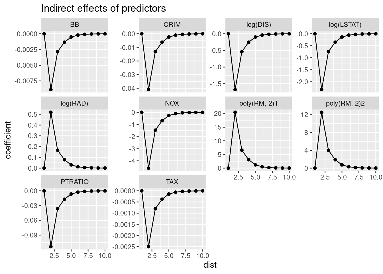
Based on the likelihood ratio test and AIC, the spatial error model is here preferable. This is also indicated by the significant residual autocorrelation of the residuals of the spatial lag model.
##          Model df    AIC  logLik
## modelErr     1 13 2665.7 -1319.8
## modelLag 2 13 2679.3 -1326.6## [1] 2679.271## [1] 2665.656To get better estimates for the uncertainty we could use a Monte Carlo Markov Chain approach based on the Metropolis random walk algorithm:
##
## Iterations = 1:1000
## Thinning interval = 1
## Number of chains = 1
## Sample size per chain = 1000
##
## 1. Empirical mean and standard deviation for each variable,
##    plus standard error of the mean:
##
##                    Mean       SD  Naive SE Time-series SE
## rho            0.398487 0.029415 9.302e-04      0.0065744
## (Intercept)   45.037503 2.900886 9.173e-02      0.6404993
## CRIM          -0.107871 0.021172 6.695e-04      0.0038825
## NOX          -11.510125 2.601767 8.228e-02      0.6278356
## poly(RM, 2)1  50.683414 4.138712 1.309e-01      0.9093784
## poly(RM, 2)2  31.830357 3.435019 1.086e-01      0.6729926
## log(DIS)      -4.199400 0.499028 1.578e-02      0.1242414
## log(RAD)       1.302632 0.300942 9.517e-03      0.0580970
## TAX           -0.005761 0.001923 6.081e-05      0.0004025
## PTRATIO       -0.315180 0.071308 2.255e-03      0.0124816
## BB            -0.024988 0.008233 2.603e-04      0.0016240
## log(LSTAT)    -5.820125 0.401025 1.268e-02      0.0832842
##
## 2. Quantiles for each variable:
##
##                    2.5%        25%        50%        75%     97.5%
## rho            0.342843   0.375410   0.404634   0.416496  0.456110
## (Intercept)   38.685042  43.548404  44.881119  46.740153 50.258197
## CRIM          -0.149575  -0.122472  -0.108894  -0.097569 -0.067206
## NOX          -17.651064 -13.538742 -11.369370 -10.026470 -6.391440
## poly(RM, 2)1  42.916325  48.310814  50.652811  53.778845 58.414160
## poly(RM, 2)2  25.013153  29.328668  31.662248  34.385886 37.734591
## log(DIS)      -5.051021  -4.553190  -4.172487  -3.796832 -3.071752
## log(RAD)       0.719926   1.093294   1.339968   1.493394  1.801804
## TAX           -0.009632  -0.007244  -0.005821  -0.004413 -0.001941
## PTRATIO       -0.468480  -0.344502  -0.320317  -0.277150 -0.162936
## BB            -0.038280  -0.030070  -0.025782  -0.020879 -0.004740
## log(LSTAT)    -6.751407  -6.085073  -5.807628  -5.506332 -5.127909
13.3.1.6 Spatial Durban error model
modelErrDurb <- spatialreg::errorsarlm(CMEDV ~ CRIM +   NOX +
                          poly(RM, 2) + log(DIS) + log(RAD) + TAX +
                          PTRATIO + BB + log(LSTAT), data = bostonSf,
                        listw = queenLw, Durbin = TRUE,
                        method = "eigen")
summary(modelErrDurb)
##
## Call:spatialreg::errorsarlm(formula = CMEDV ~ CRIM + NOX + poly(RM,
## 2) + log(DIS) + log(RAD) + TAX + PTRATIO + BB + log(LSTAT),
## data = bostonSf, listw = queenLw, Durbin = TRUE, method = "eigen")
##
## Residuals:
## Min 1Q Median 3Q Max
## -24.29889 -1.56411 -0.13454 1.39888 20.54261
##
## Type: error
## Coefficients: (asymptotic standard errors)
## Estimate Std. Error z value Pr(>|z|)
## (Intercept) 73.5704234 6.4287153 11.4440 < 2.2e-16
## CRIM -0.1092327 0.0233624 -4.6756 2.931e-06
## NOX -11.9291401 5.0292427 -2.3720 0.0176942
## poly(RM, 2)1 58.7285122 4.9981359 11.7501 < 2.2e-16
## poly(RM, 2)2 30.8189369 3.7782330 8.1570 4.441e-16
## log(DIS) -7.1151098 2.3888474 -2.9785 0.0028969
## log(RAD) 1.3254111 0.4835735 2.7409 0.0061277
## TAX -0.0091538 0.0027189 -3.3667 0.0007606
## PTRATIO -0.4190478 0.1332810 -3.1441 0.0016660
## BB -0.0518989 0.0165748 -3.1312 0.0017410
## log(LSTAT) -6.2703461 0.4864048 -12.8912 < 2.2e-16
## lag.CRIM -0.0613143 0.0576071 -1.0644 0.2871684
## lag.NOX -7.2563178 7.8128239 -0.9288 0.3530082
## lag.poly(RM, 2)1 -0.2370301 11.4068632 -0.0208 0.9834215
## lag.poly(RM, 2)2 11.7754955 8.4700808 1.3902 0.1644542
## lag.log(DIS) 1.0234149 2.6599440 0.3848 0.7004222
## lag.log(RAD) 0.4731986 0.9219095 0.5133 0.6077548
## lag.TAX 0.0030034 0.0051373 0.5846 0.5587962
## lag.PTRATIO -0.1188579 0.2287384 -0.5196 0.6033257
## lag.BB 0.0252705 0.0257465 0.9815 0.3263409
## lag.log(LSTAT) -3.5666067 1.0099832 -3.5314 0.0004134
##
## Lambda: 0.61391, LR test value: 129.99, p-value: < 2.22e-16
## Asymptotic standard error: 0.043494
## z-value: 14.115, p-value: < 2.22e-16
## Wald statistic: 199.23, p-value: < 2.22e-16
##
## Log likelihood: -1304.408 for error model
## ML residual variance (sigma squared): 9.2417, (sigma: 3.04)
## Number of observations: 506
## Number of parameters estimated: 23
## AIC: 2654.8, (AIC for lm: 2782.8)Simplifying the SLX part:
modelErrDurb <- spatialreg::errorsarlm(CMEDV ~ CRIM +   NOX +
                          poly(RM, 2) + log(DIS) + log(RAD) + TAX +
                          PTRATIO + BB + log(LSTAT), data = bostonSf,
                        listw = queenLw, Durbin = ~ CRIM +   NOX +
                          poly(RM, 2) + log(RAD) + TAX +
                          PTRATIO + BB + log(LSTAT),
                        method = "eigen")
summary(modelErrDurb)
##
## Call:spatialreg::errorsarlm(formula = CMEDV ~ CRIM + NOX + poly(RM,
## 2) + log(DIS) + log(RAD) + TAX + PTRATIO + BB + log(LSTAT),
## data = bostonSf, listw = queenLw, Durbin = ~CRIM + NOX +
## poly(RM, 2) + log(RAD) + TAX + PTRATIO + BB + log(LSTAT),
## method = "eigen")
##
## Residuals:
## Min 1Q Median 3Q Max
## -24.40308 -1.61558 -0.13942 1.38588 20.58848
##
## Type: error
## Coefficients: (asymptotic standard errors)
## Estimate Std. Error z value Pr(>|z|)
## (Intercept) 74.3240960 6.1238377 12.1368 < 2.2e-16
## CRIM -0.1088838 0.0233481 -4.6635 3.109e-06
## NOX -11.8404728 5.0247267 -2.3564 0.0184510
## poly(RM, 2)1 58.5530326 4.9780369 11.7623 < 2.2e-16
## poly(RM, 2)2 30.7926045 3.7781532 8.1502 4.441e-16
## log(DIS) -6.3077029 1.1414831 -5.5259 3.278e-08
## log(RAD) 1.3276586 0.4836124 2.7453 0.0060457
## TAX -0.0092294 0.0027122 -3.4030 0.0006666
## PTRATIO -0.4179837 0.1332728 -3.1363 0.0017109
## BB -0.0516575 0.0165655 -3.1184 0.0018185
## log(LSTAT) -6.2863872 0.4846863 -12.9700 < 2.2e-16
## lag.CRIM -0.0630018 0.0574486 -1.0967 0.2727882
## lag.NOX -8.0217154 7.5562828 -1.0616 0.2884194
## lag.poly(RM, 2)1 -0.3753368 11.4027085 -0.0329 0.9737412
## lag.poly(RM, 2)2 11.3535556 8.3998418 1.3516 0.1764908
## lag.log(RAD) 0.4934696 0.9205334 0.5361 0.5919107
## lag.TAX 0.0029419 0.0051355 0.5729 0.5667374
## lag.PTRATIO -0.1239135 0.2283922 -0.5425 0.5874418
## lag.BB 0.0249905 0.0257396 0.9709 0.3315992
## lag.log(LSTAT) -3.5645031 1.0100967 -3.5289 0.0004173
##
## Lambda: 0.61388, LR test value: 130.14, p-value: < 2.22e-16
## Asymptotic standard error: 0.043496
## z-value: 14.114, p-value: < 2.22e-16
## Wald statistic: 199.19, p-value: < 2.22e-16
##
## Log likelihood: -1304.482 for error model
## ML residual variance (sigma squared): 9.2445, (sigma: 3.0405)
## Number of observations: 506
## Number of parameters estimated: 22
## AIC: 2653, (AIC for lm: 2781.1)modelErrDurb <- spatialreg::errorsarlm(CMEDV ~ CRIM + NOX +
poly(RM, 2) + log(DIS) + log(RAD) + TAX +
PTRATIO + BB + log(LSTAT), data = bostonSf,
listw = queenLw, Durbin = ~ CRIM + NOX +
poly(RM, 2) + log(RAD) + TAX + BB + log(LSTAT),
method = "eigen")
summary(modelErrDurb)##
## Call:spatialreg::errorsarlm(formula = CMEDV ~ CRIM + NOX + poly(RM,
## 2) + log(DIS) + log(RAD) + TAX + PTRATIO + BB + log(LSTAT),
## data = bostonSf, listw = queenLw, Durbin = ~CRIM + NOX +
## poly(RM, 2) + log(RAD) + TAX + BB + log(LSTAT), method = "eigen")
##
## Residuals:
## Min 1Q Median 3Q Max
## -24.37485 -1.63636 -0.16319 1.37100 20.63212
##
## Type: error
## Coefficients: (asymptotic standard errors)
## Estimate Std. Error z value Pr(>|z|)
## (Intercept) 72.4949142 5.1339173 14.1208 < 2.2e-16
## CRIM -0.1087991 0.0233567 -4.6581 3.191e-06
## NOX -12.0425940 5.0083564 -2.4045 0.0161946
## poly(RM, 2)1 58.6871933 4.9749595 11.7965 < 2.2e-16
## poly(RM, 2)2 30.8777010 3.7757117 8.1780 2.220e-16
## log(DIS) -6.2361534 1.1377096 -5.4813 4.222e-08
## log(RAD) 1.3600807 0.4798176 2.8346 0.0045886
## TAX -0.0090597 0.0026926 -3.3646 0.0007666
## PTRATIO -0.4494914 0.1197290 -3.7542 0.0001739
## BB -0.0515165 0.0165586 -3.1112 0.0018635
## log(LSTAT) -6.2640626 0.4830083 -12.9689 < 2.2e-16
## lag.CRIM -0.0615568 0.0574942 -1.0707 0.2843216
## lag.NOX -7.0437931 7.3438084 -0.9591 0.3374846
## lag.poly(RM, 2)1 0.6245389 11.2854943 0.0553 0.9558676
## lag.poly(RM, 2)2 12.0603163 8.3013232 1.4528 0.1462741
## lag.log(RAD) 0.4188893 0.9127297 0.4589 0.6462763
## lag.TAX 0.0023049 0.0049960 0.4613 0.6445528
## lag.BB 0.0249366 0.0257713 0.9676 0.3332375
## lag.log(LSTAT) -3.6416957 1.0018256 -3.6351 0.0002779
##
## Lambda: 0.6161, LR test value: 131.97, p-value: < 2.22e-16
## Asymptotic standard error: 0.043347
## z-value: 14.213, p-value: < 2.22e-16
## Wald statistic: 202.01, p-value: < 2.22e-16
##
## Log likelihood: -1304.628 for error model
## ML residual variance (sigma squared): 9.2422, (sigma: 3.0401)
## Number of observations: 506
## Number of parameters estimated: 21
## AIC: 2651.3, (AIC for lm: 2781.2)modelErrDurb <- spatialreg::errorsarlm(CMEDV ~ CRIM + NOX +
poly(RM, 2) + log(DIS) + log(RAD) + TAX +
PTRATIO + BB + log(LSTAT), data = bostonSf,
listw = queenLw, Durbin = ~ CRIM + NOX +
poly(RM, 2) + log(RAD) +
BB + log(LSTAT),
method = "eigen")
summary(modelErrDurb)##
## Call:spatialreg::errorsarlm(formula = CMEDV ~ CRIM + NOX + poly(RM,
## 2) + log(DIS) + log(RAD) + TAX + PTRATIO + BB + log(LSTAT),
## data = bostonSf, listw = queenLw, Durbin = ~CRIM + NOX +
## poly(RM, 2) + log(RAD) + BB + log(LSTAT), method = "eigen")
##
## Residuals:
## Min 1Q Median 3Q Max
## -24.42674 -1.63351 -0.15519 1.41901 20.62695
##
## Type: error
## Coefficients: (asymptotic standard errors)
## Estimate Std. Error z value Pr(>|z|)
## (Intercept) 72.6328619 5.1171797 14.1939 < 2.2e-16
## CRIM -0.1085638 0.0233526 -4.6489 3.337e-06
## NOX -12.3520126 4.9678050 -2.4864 0.0129038
## poly(RM, 2)1 58.6798893 4.9754440 11.7939 < 2.2e-16
## poly(RM, 2)2 30.8937788 3.7760994 8.1814 2.220e-16
## log(DIS) -6.2879671 1.1295946 -5.5666 2.598e-08
## log(RAD) 1.3198539 0.4719550 2.7966 0.0051649
## TAX -0.0086104 0.0025124 -3.4271 0.0006100
## PTRATIO -0.4505267 0.1196603 -3.7650 0.0001665
## BB -0.0513536 0.0165659 -3.1000 0.0019355
## log(LSTAT) -6.2684505 0.4830298 -12.9774 < 2.2e-16
## lag.CRIM -0.0589797 0.0571125 -1.0327 0.3017480
## lag.NOX -6.3864982 7.2006803 -0.8869 0.3751167
## lag.poly(RM, 2)1 0.2757975 11.2555569 0.0245 0.9804512
## lag.poly(RM, 2)2 11.7316500 8.2632775 1.4197 0.1556853
## lag.log(RAD) 0.7010596 0.6795635 1.0316 0.3022445
## lag.BB 0.0255110 0.0257308 0.9915 0.3214634
## lag.log(LSTAT) -3.6202833 0.9998460 -3.6208 0.0002936
##
## Lambda: 0.61437, LR test value: 132.09, p-value: < 2.22e-16
## Asymptotic standard error: 0.043463
## z-value: 14.136, p-value: < 2.22e-16
## Wald statistic: 199.81, p-value: < 2.22e-16
##
## Log likelihood: -1304.733 for error model
## ML residual variance (sigma squared): 9.252, (sigma: 3.0417)
## Number of observations: 506
## Number of parameters estimated: 20
## AIC: 2649.5, (AIC for lm: 2779.6)modelErrDurb <- spatialreg::errorsarlm(CMEDV ~ CRIM + ZN + NOX +
poly(RM, 2) + log(DIS) + log(RAD) + TAX +
PTRATIO + BB + log(LSTAT), data = bostonSf,
listw = queenLw, Durbin = ~ CRIM + ZN + NOX +
poly(RM, 2) + log(RAD) +
log(LSTAT),
method = "eigen")
summary(modelErrDurb)##
## Call:spatialreg::errorsarlm(formula = CMEDV ~ CRIM + ZN + NOX + poly(RM,
## 2) + log(DIS) + log(RAD) + TAX + PTRATIO + BB + log(LSTAT),
## data = bostonSf, listw = queenLw, Durbin = ~CRIM + ZN + NOX +
## poly(RM, 2) + log(RAD) + log(LSTAT), method = "eigen")
##
## Residuals:
## Min 1Q Median 3Q Max
## -24.31751 -1.56408 -0.13862 1.38515 20.43384
##
## Type: error
## Coefficients: (asymptotic standard errors)
## Estimate Std. Error z value Pr(>|z|)
## (Intercept) 71.5479621 5.1348662 13.9338 < 2.2e-16
## CRIM -0.1082179 0.0234120 -4.6223 3.795e-06
## ZN 0.0216262 0.0112004 1.9308 0.0535031
## NOX -10.7629301 5.0333011 -2.1383 0.0324888
## poly(RM, 2)1 58.9795328 4.9637729 11.8820 < 2.2e-16
## poly(RM, 2)2 30.6562778 3.7688893 8.1340 4.441e-16
## log(DIS) -6.6030524 1.2508986 -5.2786 1.301e-07
## log(RAD) 1.3680891 0.4726085 2.8948 0.0037945
## TAX -0.0089655 0.0025756 -3.4810 0.0004996
## PTRATIO -0.3972247 0.1242689 -3.1965 0.0013911
## BB -0.0433456 0.0140651 -3.0818 0.0020577
## log(LSTAT) -6.1276980 0.4876519 -12.5657 < 2.2e-16
## lag.CRIM -0.0568910 0.0577253 -0.9855 0.3243557
## lag.ZN -0.0108111 0.0216960 -0.4983 0.6182741
## lag.NOX -7.9169439 7.2570769 -1.0909 0.2753048
## lag.poly(RM, 2)1 1.2783566 11.3211617 0.1129 0.9100960
## lag.poly(RM, 2)2 10.8978986 8.2843711 1.3155 0.1883497
## lag.log(RAD) 0.7300391 0.6856287 1.0648 0.2869786
## lag.log(LSTAT) -3.5849904 1.0046767 -3.5683 0.0003593
##
## Lambda: 0.61923, LR test value: 133.78, p-value: < 2.22e-16
## Asymptotic standard error: 0.043135
## z-value: 14.356, p-value: < 2.22e-16
## Wald statistic: 206.09, p-value: < 2.22e-16
##
## Log likelihood: -1303.366 for error model
## ML residual variance (sigma squared): 9.1855, (sigma: 3.0308)
## Number of observations: 506
## Number of parameters estimated: 21
## AIC: 2648.7, (AIC for lm: 2780.5)modelErrDurb <- spatialreg::errorsarlm(CMEDV ~ CRIM + NOX +
poly(RM, 2) + log(DIS) + log(RAD) + TAX +
PTRATIO + BB + log(LSTAT), data = bostonSf,
listw = queenLw, Durbin = ~ CRIM + NOX +
poly(RM, 2) +
log(LSTAT),
method = "eigen")
summary(modelErrDurb)##
## Call:spatialreg::errorsarlm(formula = CMEDV ~ CRIM + NOX + poly(RM,
## 2) + log(DIS) + log(RAD) + TAX + PTRATIO + BB + log(LSTAT),
## data = bostonSf, listw = queenLw, Durbin = ~CRIM + NOX +
## poly(RM, 2) + log(LSTAT), method = "eigen")
##
## Residuals:
## Min 1Q Median 3Q Max
## -24.71398 -1.60027 -0.15928 1.30019 20.38419
##
## Type: error
## Coefficients: (asymptotic standard errors)
## Estimate Std. Error z value Pr(>|z|)
## (Intercept) 72.0996596 5.1424598 14.0205 < 2.2e-16
## CRIM -0.1057065 0.0233359 -4.5298 5.904e-06
## NOX -13.7889302 4.8444491 -2.8463 0.0044225
## poly(RM, 2)1 58.7336613 4.9847077 11.7828 < 2.2e-16
## poly(RM, 2)2 30.8443114 3.7791854 8.1616 2.220e-16
## log(DIS) -6.1930552 1.1393884 -5.4354 5.467e-08
## log(RAD) 1.5159718 0.4371700 3.4677 0.0005249
## TAX -0.0081460 0.0025002 -3.2581 0.0011216
## PTRATIO -0.4600347 0.1198999 -3.8368 0.0001246
## BB -0.0418538 0.0141085 -2.9666 0.0030115
## log(LSTAT) -6.2719581 0.4839805 -12.9591 < 2.2e-16
## lag.CRIM -0.0298993 0.0537684 -0.5561 0.5781593
## lag.NOX -3.1931580 6.7726663 -0.4715 0.6373000
## lag.poly(RM, 2)1 2.2458791 11.2499126 0.1996 0.8417659
## lag.poly(RM, 2)2 11.5577437 8.2849875 1.3950 0.1630091
## lag.log(LSTAT) -3.4629961 0.9997342 -3.4639 0.0005324
##
## Lambda: 0.62005, LR test value: 134.57, p-value: < 2.22e-16
## Asymptotic standard error: 0.04308
## z-value: 14.393, p-value: < 2.22e-16
## Wald statistic: 207.16, p-value: < 2.22e-16
##
## Log likelihood: -1305.842 for error model
## ML residual variance (sigma squared): 9.2731, (sigma: 3.0452)
## Number of observations: 506
## Number of parameters estimated: 18
## AIC: 2647.7, (AIC for lm: 2780.3)modelErrDurb <- spatialreg::errorsarlm(CMEDV ~ CRIM + NOX +
poly(RM, 2) + log(DIS) + log(RAD) + TAX +
PTRATIO + BB + log(LSTAT), data = bostonSf,
listw = queenLw, Durbin = ~ CRIM + NOX +
log(LSTAT),
method = "eigen")
summary(modelErrDurb)##
## Call:spatialreg::errorsarlm(formula = CMEDV ~ CRIM + NOX + poly(RM,
## 2) + log(DIS) + log(RAD) + TAX + PTRATIO + BB + log(LSTAT),
## data = bostonSf, listw = queenLw, Durbin = ~CRIM + NOX +
## log(LSTAT), method = "eigen")
##
## Residuals:
## Min 1Q Median 3Q Max
## -24.06664 -1.66062 -0.16977 1.32049 20.44091
##
## Type: error
## Coefficients: (asymptotic standard errors)
## Estimate Std. Error z value Pr(>|z|)
## (Intercept) 73.3335112 4.7953570 15.2926 < 2.2e-16
## CRIM -0.1060624 0.0233449 -4.5433 5.538e-06
## NOX -13.2093485 4.8344771 -2.7323 0.0062890
## poly(RM, 2)1 58.7480552 4.9727010 11.8141 < 2.2e-16
## poly(RM, 2)2 30.2086897 3.7600324 8.0342 8.882e-16
## log(DIS) -6.4482896 1.1320345 -5.6962 1.225e-08
## log(RAD) 1.5162769 0.4388033 3.4555 0.0005493
## TAX -0.0081473 0.0025085 -3.2479 0.0011627
## PTRATIO -0.4763920 0.1190261 -4.0024 6.270e-05
## BB -0.0437594 0.0140137 -3.1226 0.0017925
## log(LSTAT) -6.3514221 0.4799504 -13.2335 < 2.2e-16
## lag.CRIM -0.0156266 0.0530346 -0.2947 0.7682610
## lag.NOX -3.5806752 6.8006907 -0.5265 0.5985295
## lag.log(LSTAT) -3.7093032 0.7940582 -4.6713 2.993e-06
##
## Lambda: 0.62578, LR test value: 139.56, p-value: < 2.22e-16
## Asymptotic standard error: 0.042689
## z-value: 14.659, p-value: < 2.22e-16
## Wald statistic: 214.89, p-value: < 2.22e-16
##
## Log likelihood: -1306.806 for error model
## ML residual variance (sigma squared): 9.2883, (sigma: 3.0477)
## Number of observations: 506
## Number of parameters estimated: 16
## AIC: 2645.6, (AIC for lm: 2783.2)modelErrDurb <- spatialreg::errorsarlm(CMEDV ~ CRIM + NOX +
poly(RM, 2) + log(DIS) + log(RAD) + TAX +
PTRATIO + BB + log(LSTAT), data = bostonSf,
listw = queenLw, Durbin = ~ NOX +
log(LSTAT),
method = "eigen")
summary(modelErrDurb)##
## Call:spatialreg::errorsarlm(formula = CMEDV ~ CRIM + NOX + poly(RM,
## 2) + log(DIS) + log(RAD) + TAX + PTRATIO + BB + log(LSTAT),
## data = bostonSf, listw = queenLw, Durbin = ~NOX + log(LSTAT),
## method = "eigen")
##
## Residuals:
## Min 1Q Median 3Q Max
## -24.02137 -1.63105 -0.14231 1.32385 20.43556
##
## Type: error
## Coefficients: (asymptotic standard errors)
## Estimate Std. Error z value Pr(>|z|)
## (Intercept) 73.3376684 4.8039577 15.2661 < 2.2e-16
## CRIM -0.1052890 0.0232158 -4.5352 5.754e-06
## NOX -13.0860254 4.8181354 -2.7160 0.0066077
## poly(RM, 2)1 58.6514349 4.9598970 11.8251 < 2.2e-16
## poly(RM, 2)2 30.1909424 3.7598767 8.0298 8.882e-16
## log(DIS) -6.3922193 1.1176820 -5.7192 1.070e-08
## log(RAD) 1.5017750 0.4367215 3.4387 0.0005844
## TAX -0.0082519 0.0024859 -3.3195 0.0009018
## PTRATIO -0.4748912 0.1190428 -3.9892 6.628e-05
## BB -0.0445428 0.0137964 -3.2286 0.0012440
## log(LSTAT) -6.3644808 0.4778283 -13.3196 < 2.2e-16
## lag.NOX -3.6036219 6.8063526 -0.5294 0.5964935
## lag.log(LSTAT) -3.7545284 0.7804677 -4.8106 1.505e-06
##
## Lambda: 0.62722, LR test value: 143.06, p-value: < 2.22e-16
## Asymptotic standard error: 0.04259
## z-value: 14.727, p-value: < 2.22e-16
## Wald statistic: 216.88, p-value: < 2.22e-16
##
## Log likelihood: -1306.849 for error model
## ML residual variance (sigma squared): 9.2848, (sigma: 3.0471)
## Number of observations: 506
## Number of parameters estimated: 15
## AIC: 2643.7, (AIC for lm: 2784.8)modelErrDurb <- spatialreg::errorsarlm(CMEDV ~ CRIM + NOX +
poly(RM, 2) + log(DIS) + log(RAD) + TAX +
PTRATIO + BB + log(LSTAT), data = bostonSf,
listw = queenLw, Durbin = ~ log(LSTAT),
method = "eigen")
summary(modelErrDurb)##
## Call:spatialreg::errorsarlm(formula = CMEDV ~ CRIM + NOX + poly(RM,
## 2) + log(DIS) + log(RAD) + TAX + PTRATIO + BB + log(LSTAT),
## data = bostonSf, listw = queenLw, Durbin = ~log(LSTAT), method = "eigen")
##
## Residuals:
## Min 1Q Median 3Q Max
## -24.16522 -1.63291 -0.16465 1.33719 20.41922
##
## Type: error
## Coefficients: (asymptotic standard errors)
## Estimate Std. Error z value Pr(>|z|)
## (Intercept) 71.9165468 3.9833723 18.0542 < 2.2e-16
## CRIM -0.1050493 0.0232180 -4.5245 6.055e-06
## NOX -14.4125581 4.1179474 -3.4999 0.0004654
## poly(RM, 2)1 58.3659792 4.9321950 11.8337 < 2.2e-16
## poly(RM, 2)2 29.9209876 3.7257071 8.0310 8.882e-16
## log(DIS) -6.0803475 0.9498874 -6.4011 1.542e-10
## log(RAD) 1.5026964 0.4368044 3.4402 0.0005813
## TAX -0.0082334 0.0024862 -3.3117 0.0009274
## PTRATIO -0.4712111 0.1188559 -3.9646 7.353e-05
## BB -0.0447002 0.0137948 -3.2404 0.0011938
## log(LSTAT) -6.3755722 0.4775124 -13.3516 < 2.2e-16
## lag.log(LSTAT) -3.8675465 0.7507233 -5.1518 2.581e-07
##
## Lambda: 0.62701, LR test value: 142.86, p-value: < 2.22e-16
## Asymptotic standard error: 0.042605
## z-value: 14.717, p-value: < 2.22e-16
## Wald statistic: 216.58, p-value: < 2.22e-16
##
## Log likelihood: -1306.989 for error model
## ML residual variance (sigma squared): 9.2907, (sigma: 3.0481)
## Number of observations: 506
## Number of parameters estimated: 14
## AIC: 2642, (AIC for lm: 2782.8)Only the share of the lower status population stayed in as a lagged predictor.
##              Model df    AIC  logLik Test L.Ratio   p-value
## modelErr         1 13 2665.7 -1319.8    1
## modelErrDurb     2 14 2642.0 -1307.0    2  25.678 4.033e-07
This inclusion of the lagged predictor led to a significantly better model according to the LR test and to the AIC.
## [1] 2665.656## [1] 2641.978Let’s compare the regression coefficient of the spatial error model with and without the lagged predictors:
##        lambda   (Intercept)          CRIM           NOX  poly(RM, 2)1
##   0.646316338  64.281505852  -0.117714109 -16.834542627  58.131692051
##  poly(RM, 2)2      log(DIS)      log(RAD)           TAX       PTRATIO
##  31.474124677  -4.669359219   1.481673647  -0.008283067  -0.522592916
##            BB    log(LSTAT)
## -0.049894964 -6.711161116## lambda (Intercept) CRIM NOX poly(RM, 2)1
## 0.627005748 71.916546803 -0.105049307 -14.412558079 58.365979208
## poly(RM, 2)2 log(DIS) log(RAD) TAX PTRATIO
## 29.920987614 -6.080347541 1.502696397 -0.008233407 -0.471211110
## BB log(LSTAT) lag.log(LSTAT)
## -0.044700165 -6.375572208 -3.867546458The sign of the coefficients did not change, however, the see some change in the size of the coefficients, which become more obvious if the compare by mean of a division (coefficient error model with lagged predictors / coefficient error model):
## lambda (Intercept) CRIM NOX poly(RM, 2)1 poly(RM, 2)2
## 0.029877924 -0.118775079 0.107589500 0.143869935 -0.004030283 0.049346474
## log(DIS) log(RAD) TAX PTRATIO BB log(LSTAT)
## -0.302180290 -0.014188516 0.005995346 0.098320901 0.104114685 0.050004597The coefficient for NOX is increased by 14%, the coefficient for weighted distances to five Boston employment centers(log(DIS)) is reduced by 30%, effect of crime rate per person, share of black population and for pupil-teacher ratio (PRATIO) is increased by around 10%.
13.3.1.7 Spatialy lagged predictor model
We should also try, maybe before moving to the lag and error models a spatially lagged predictor (SLX) model. The model can be run using spatialreg::lmLSX or by simply creating the lagged predictors and attaching them to the data.frame and then using a normal linear model by lm (or glm or other regression models such as tree based approaches).
modelSLX <- spatialreg::lmSLX(CMEDV ~ CRIM + ZN + CHAS + poly(NOX, 2) + poly(RM,2) +
log(DIS) + log(RAD) + TAX + PTRATIO + BB + log(LSTAT),
data = bostonSf,
listw = queenLw,
Durbin= TRUE)
summary(modelSLX)##
## Call:
## lm(formula = formula(paste("y ~ ", paste(colnames(x)[-1], collapse = "+"))),
## data = as.data.frame(x), weights = weights)
##
## Coefficients:
## Estimate Std. Error t value Pr(>|t|)
## (Intercept) 6.397e+01 3.098e+00 2.065e+01 3.309e-68
## CRIM -1.083e-01 2.794e-02 -3.876e+00 1.208e-04
## ZN 2.174e-02 1.517e-02 1.433e+00 1.524e-01
## CHAS1 -1.247e+00 9.952e-01 -1.253e+00 2.109e-01
## poly.NOX..2.1 -3.019e+01 1.951e+01 -1.548e+00 1.223e-01
## poly.NOX..2.2 -1.211e+00 1.176e+01 -1.029e-01 9.181e-01
## poly.RM..2.1 5.811e+01 6.030e+00 9.638e+00 3.287e-20
## poly.RM..2.2 3.194e+01 4.476e+00 7.136e+00 3.575e-12
## log.DIS. -8.913e+00 3.288e+00 -2.711e+00 6.944e-03
## log.RAD. 1.014e+00 6.214e-01 1.632e+00 1.033e-01
## TAX -8.342e-03 3.547e-03 -2.352e+00 1.908e-02
## PTRATIO -2.823e-01 1.740e-01 -1.622e+00 1.054e-01
## BB -5.809e-02 2.137e-02 -2.718e+00 6.800e-03
## log.LSTAT. -6.347e+00 6.054e-01 -1.048e+01 2.727e-23
## lag.CRIM -1.225e-01 5.390e-02 -2.272e+00 2.351e-02
## lag.ZN 7.284e-03 2.330e-02 3.126e-01 7.547e-01
## lag.CHAS1 6.113e+00 1.453e+00 4.206e+00 3.101e-05
## lag.poly.NOX..2.1 -1.011e+01 2.330e+01 -4.340e-01 6.645e-01
## lag.poly.NOX..2.2 -2.051e+01 1.412e+01 -1.452e+00 1.471e-01
## lag.poly.RM..2.1 -1.864e+01 1.066e+01 -1.748e+00 8.107e-02
## lag.poly.RM..2.2 1.202e+01 8.261e+00 1.455e+00 1.464e-01
## lag.log.DIS. 3.795e+00 3.462e+00 1.096e+00 2.735e-01
## lag.log.RAD. 8.400e-01 9.409e-01 8.927e-01 3.725e-01
## lag.TAX 2.808e-03 5.440e-03 5.163e-01 6.059e-01
## lag.PTRATIO -4.768e-01 2.434e-01 -1.959e+00 5.072e-02
## lag.BB 4.751e-02 2.703e-02 1.758e+00 7.941e-02
## lag.log.LSTAT. -3.065e+00 9.606e-01 -3.190e+00 1.515e-03Or alternatively, we could create the predictors we would like to include manually. We would then have to attach them to the data frame.
## [1] 9.867510 13.463610 10.447347 11.523269 9.284115 12.302833 10.194769
## [8] 11.179965 9.309884 8.470902 12.764990 12.518008 9.202269 6.749474
## [15] 11.735829 6.010698 16.298210 37.970000 27.983174 21.180026 17.044693
## [22] 20.857104 18.234974 21.960281 25.028525 21.842572 24.715557 28.478894
## [29] 27.168620 28.803702 29.931054 27.904516 27.682519 22.712915 18.351138
## [36] 13.394860 22.551587 21.771823 17.262927 17.701239 19.186725 20.431728
## [43] 21.838115 24.190130 24.137534 24.317222 22.570125 24.219103 24.499773
## [50] 27.957416 12.130000 13.974651 21.690976 21.611840 17.237620 22.149338
## [57] 22.266288 29.066018 26.973597 30.585743 26.842413 24.087229 22.242450
## [64] 18.177135 20.930153 12.941595 18.438447 18.034509 21.352705 17.583457
## [71] 18.952296 20.938331 19.278221 23.804900 18.083051 17.573338 17.949731
## [78] 16.613224 18.243746 19.278986 23.884394 24.573447 28.009001 25.239047
## [85] 20.302101 17.499052 20.094605 20.907792 26.298449 21.215697 19.630125
## [92] 18.268316 17.819129 18.776393 17.439166 17.489644 16.323592 17.582645
## [99] 17.340232 18.046900 17.584967 17.031422 16.368318 14.262988 16.374535
## [106] 14.166939 11.338756 13.046437 11.695863 14.509012 16.862106 16.818418
## [113] 15.451760 18.330530 15.137409 12.656944 11.429613 14.364425 19.258141
## [120] 20.039221 19.259934 20.019597 20.142215 17.750397 7.285227 10.218574
## [127] 11.301427 10.310671 12.408867 11.065400 11.451443 14.765924 21.413475
## [134] 22.826069 19.365283 17.844891 17.294173 14.002263 14.749600 13.548142
## [141] 14.035965 16.065053 15.359817 15.959097 14.744397 10.815599 9.904220
## [148] 13.443954 8.299462 6.990915 17.625076 11.155349 9.267335 7.565076
## [155] 10.687002 15.572399 12.508343 21.840250 14.751978 17.550274 17.864769
## [162] 17.780805 15.101046 12.841409 13.069804 11.028860 9.303931 14.489765
## [169] 10.046416 13.396594 15.985536 16.418404 18.156963 19.828804 17.907464
## [176] 15.231858 13.492326 14.883629 12.848201 15.119320 17.257922 19.484918
## [183] 17.600501 21.208875 19.630743 15.527963 11.478195 9.336346 8.408377
## [190] 8.177952 7.493555 7.017264 4.753191 8.158433 16.535790 9.293402
## [197] 12.765691 18.826121 14.739833 18.302028 10.402215 9.495971 8.351989
## [204] 7.265291 5.136167 7.264095 4.950818 6.603016 9.142490 12.157504
## [211] 9.199576 13.702346 12.841084 6.572931 7.157715 8.124335 6.792014
## [218] 9.462819 8.355800 8.922136 8.086985 8.271023 7.349252 5.700771
## [225] 6.372239 9.586658 9.449895 9.643194 9.232348 9.107374 7.917100
## [232] 6.510576 7.707659 6.617470 7.379914 8.415247 7.076560 7.703828
## [239] 7.525037 8.121367 10.764584 10.126465 8.047780 8.549995 7.683908
## [246] 9.778936 7.513626 8.579909 6.299858 7.679365 11.776625 9.616360
## [253] 10.601907 11.564729 13.689925 15.156725 14.596025 17.852097 14.118514
## [260] 11.857835 12.835378 13.475556 12.383847 11.968491 16.764671 12.987729
## [267] 13.297589 12.662953 13.478048 13.425229 14.746981 16.232990 17.015329
## [274] 16.922458 17.363375 19.563341 19.920404 19.464820 17.841926 15.091503
## [281] 14.782755 14.868325 13.861872 11.890637 12.995987 13.400396 12.860193
## [288] 17.812063 16.578133 22.462010 21.552068 23.425004 19.418525 29.648445
## [295] 27.551192 22.356414 21.646711 24.902266 25.378082 22.781833 15.829434
## [302] 14.711226 14.691188 12.219915 13.727893 13.243291 9.175417 9.027244
## [309] 7.718087 11.997259 11.341681 3.959159 5.956098 9.920029 9.988903
## [316] 8.918509 7.374459 9.853852 13.101512 12.474266 11.552186 14.120558
## [323] 9.898508 11.363532 9.993801 7.845451 5.627570 7.070193 8.038538
## [330] 8.597906 7.704439 10.002270 7.923173 8.516547 9.772950 11.537099
## [337] 8.415512 7.371564 10.659217 5.431001 5.934559 3.731784 5.637621
## [344] 5.113028 5.030000 6.245333 5.715117 4.799402 4.799215 5.067337
## [351] 3.733876 6.319389 4.563520 7.755908 7.751265 10.143038 9.851942
## [358] 11.255596 15.613898 18.945015 15.663595 15.963757 16.758870 17.327131
## [365] 10.027840 17.302701 13.730683 9.799975 10.433923 11.834859 11.637031
## [372] 11.094392 11.355702 6.188489 7.856333 6.193800 5.553296 4.187878
## [379] 5.799986 6.974483 4.930570 5.442113 5.716005 5.728166 12.249070
## [386] 12.858561 10.897220 6.069179 6.518942 7.432503 6.850683 8.250241
## [393] 7.398293 9.440587 11.039975 9.534685 10.356437 10.515018 7.316299
## [400] 6.485222 6.004210 5.629765 5.523637 7.279609 9.127269 11.270849
## [407] 10.356443 9.057374 8.244611 9.155186 7.782879 8.957421 9.242410
## [414] 9.228810 9.750933 12.664041 10.739381 9.506592 8.808309 9.025762
## [421] 9.690296 8.006080 9.525165 7.495712 6.626733 5.324267 3.897513
## [428] 4.529442 5.709605 5.738962 4.259776 5.552647 5.683154 5.738205
## [435] 7.613812 8.218420 8.144865 8.328609 9.667491 7.233663 6.618352
## [442] 5.015859 7.045876 8.762260 6.253631 7.010664 8.506165 7.416578
## [449] 8.122630 5.610388 6.106968 6.671035 7.665636 7.659032 8.355093
## [456] 10.701342 10.938898 9.958910 9.673664 10.573094 13.120019 10.634402
## [463] 9.895498 9.095228 12.049364 11.188966 11.474134 10.498101 9.776546
## [470] 9.239770 12.083721 9.249705 9.869619 10.610714 8.293795 7.206139
## [477] 8.150028 8.054121 9.799941 8.748396 8.739736 8.418247 8.301247
## [484] 6.946078 8.091305 7.717179 8.385287 8.177775 9.366672 10.941533
## [491] 10.610429 6.388942 7.613579 7.934958 7.998383 9.709219 7.208587
## [498] 9.110599 6.810160 5.556959 6.083481 6.461093 5.192923 6.806482
## [505] 5.630768 6.990559Drop the lagged effect of TAX
modelSLX <- spatialreg::lmSLX(CMEDV ~ CRIM + ZN + CHAS + poly(NOX, 2) + poly(RM,
2) + log(DIS) + log(RAD) + TAX + PTRATIO + BB + log(LSTAT),
data = bostonSf,
Durbin = ~ CRIM + ZN + CHAS + poly(NOX, 2) + poly(RM,2) + log(DIS) + log(RAD) + PTRATIO + BB + log(LSTAT),
listw = queenLw)
summary(modelSLX)##
## Call:
## lm(formula = formula(paste("y ~ ", paste(colnames(x)[-1], collapse = "+"))),
## data = as.data.frame(x), weights = weights)
##
## Coefficients:
## Estimate Std. Error t value Pr(>|t|)
## (Intercept) 6.400e+01 3.096e+00 2.067e+01 2.208e-68
## CRIM -1.091e-01 2.787e-02 -3.914e+00 1.039e-04
## ZN 2.112e-02 1.511e-02 1.398e+00 1.628e-01
## CHAS1 -1.239e+00 9.943e-01 -1.246e+00 2.135e-01
## poly.NOX..2.1 -3.290e+01 1.877e+01 -1.753e+00 8.023e-02
## poly.NOX..2.2 -2.029e-01 1.159e+01 -1.751e-02 9.860e-01
## poly.RM..2.1 5.824e+01 6.020e+00 9.674e+00 2.431e-20
## poly.RM..2.2 3.200e+01 4.471e+00 7.158e+00 3.096e-12
## log.DIS. -8.989e+00 3.282e+00 -2.739e+00 6.388e-03
## log.RAD. 9.182e-01 5.924e-01 1.550e+00 1.218e-01
## TAX -6.984e-03 2.377e-03 -2.938e+00 3.459e-03
## PTRATIO -2.998e-01 1.705e-01 -1.759e+00 7.923e-02
## BB -5.791e-02 2.135e-02 -2.713e+00 6.917e-03
## log.LSTAT. -6.348e+00 6.049e-01 -1.049e+01 2.460e-23
## lag.CRIM -1.218e-01 5.385e-02 -2.262e+00 2.415e-02
## lag.ZN 1.030e-02 2.254e-02 4.571e-01 6.478e-01
## lag.CHAS1 6.017e+00 1.440e+00 4.178e+00 3.500e-05
## lag.poly.NOX..2.1 -6.797e+00 2.238e+01 -3.037e-01 7.615e-01
## lag.poly.NOX..2.2 -2.136e+01 1.402e+01 -1.523e+00 1.283e-01
## lag.poly.RM..2.1 -1.913e+01 1.061e+01 -1.804e+00 7.192e-02
## lag.poly.RM..2.2 1.159e+01 8.212e+00 1.411e+00 1.589e-01
## lag.log.DIS. 3.727e+00 3.457e+00 1.078e+00 2.815e-01
## lag.log.RAD. 1.123e+00 7.639e-01 1.470e+00 1.421e-01
## lag.PTRATIO -4.384e-01 2.316e-01 -1.893e+00 5.896e-02
## lag.BB 4.782e-02 2.700e-02 1.771e+00 7.716e-02
## lag.log.LSTAT. -3.075e+00 9.597e-01 -3.204e+00 1.443e-03Dropping lagged DIS
modelSLX <- spatialreg::lmSLX(CMEDV ~ CRIM + ZN + CHAS + poly(NOX, 2) + poly(RM,
2) + log(DIS) + log(RAD) + TAX + PTRATIO + BB + log(LSTAT),
data = bostonSf,
Durbin = ~ CRIM + ZN + CHAS + poly(NOX, 2) + poly(RM,2) +
log(RAD) + PTRATIO + BB + log(LSTAT),
listw = queenLw)
summary(modelSLX)##
## Call:
## lm(formula = formula(paste("y ~ ", paste(colnames(x)[-1], collapse = "+"))),
## data = as.data.frame(x), weights = weights)
##
## Coefficients:
## Estimate Std. Error t value Pr(>|t|)
## (Intercept) 6.418e+01 3.092e+00 2.076e+01 7.983e-69
## CRIM -1.069e-01 2.780e-02 -3.844e+00 1.370e-04
## ZN 1.971e-02 1.505e-02 1.309e+00 1.910e-01
## CHAS1 -1.289e+00 9.933e-01 -1.298e+00 1.949e-01
## poly.NOX..2.1 -3.040e+01 1.863e+01 -1.632e+00 1.034e-01
## poly.NOX..2.2 -1.954e+00 1.148e+01 -1.702e-01 8.649e-01
## poly.RM..2.1 5.765e+01 5.996e+00 9.614e+00 3.929e-20
## poly.RM..2.2 3.206e+01 4.472e+00 7.169e+00 2.857e-12
## log.DIS. -5.575e+00 8.596e-01 -6.485e+00 2.202e-10
## log.RAD. 9.168e-01 5.925e-01 1.547e+00 1.224e-01
## TAX -7.444e-03 2.339e-03 -3.183e+00 1.552e-03
## PTRATIO -2.963e-01 1.705e-01 -1.738e+00 8.287e-02
## BB -5.715e-02 2.134e-02 -2.678e+00 7.666e-03
## log.LSTAT. -6.416e+00 6.018e-01 -1.066e+01 5.778e-24
## lag.CRIM -1.280e-01 5.354e-02 -2.391e+00 1.719e-02
## lag.ZN 1.258e-02 2.244e-02 5.608e-01 5.752e-01
## lag.CHAS1 6.037e+00 1.441e+00 4.191e+00 3.306e-05
## lag.poly.NOX..2.1 -1.153e+01 2.195e+01 -5.255e-01 5.995e-01
## lag.poly.NOX..2.2 -1.868e+01 1.380e+01 -1.354e+00 1.764e-01
## lag.poly.RM..2.1 -1.882e+01 1.061e+01 -1.774e+00 7.669e-02
## lag.poly.RM..2.2 1.074e+01 8.176e+00 1.314e+00 1.896e-01
## lag.log.RAD. 1.212e+00 7.595e-01 1.596e+00 1.112e-01
## lag.PTRATIO -4.346e-01 2.316e-01 -1.877e+00 6.117e-02
## lag.BB 4.691e-02 2.699e-02 1.738e+00 8.288e-02
## lag.log.LSTAT. -2.978e+00 9.556e-01 -3.117e+00 1.939e-03Dropping lagged NOX
modelSLX <- spatialreg::lmSLX(CMEDV ~ CRIM + ZN + CHAS + poly(NOX, 2) + poly(RM,
2) + log(DIS) + log(RAD) + TAX + PTRATIO + BB + log(LSTAT),
data = bostonSf,
Durbin = ~ CRIM + ZN + CHAS + poly(RM,2) +
log(RAD) + PTRATIO + BB + log(LSTAT),
listw = queenLw)
summary(modelSLX)##
## Call:
## lm(formula = formula(paste("y ~ ", paste(colnames(x)[-1], collapse = "+"))),
## data = as.data.frame(x), weights = weights)
##
## Coefficients:
## Estimate Std. Error t value Pr(>|t|)
## (Intercept) 6.302e+01 3.031e+00 2.080e+01 4.579e-69
## CRIM -1.070e-01 2.784e-02 -3.845e+00 1.367e-04
## ZN 2.330e-02 1.404e-02 1.660e+00 9.760e-02
## CHAS1 -1.354e+00 9.932e-01 -1.363e+00 1.736e-01
## poly.NOX..2.1 -3.882e+01 9.313e+00 -4.168e+00 3.639e-05
## poly.NOX..2.2 -1.565e+01 5.572e+00 -2.809e+00 5.170e-03
## poly.RM..2.1 5.683e+01 5.966e+00 9.527e+00 7.872e-20
## poly.RM..2.2 3.136e+01 4.451e+00 7.046e+00 6.379e-12
## log.DIS. -5.351e+00 7.886e-01 -6.786e+00 3.377e-11
## log.RAD. 9.969e-01 5.633e-01 1.770e+00 7.741e-02
## TAX -7.459e-03 2.323e-03 -3.211e+00 1.410e-03
## PTRATIO -3.205e-01 1.687e-01 -1.899e+00 5.812e-02
## BB -5.507e-02 2.134e-02 -2.580e+00 1.016e-02
## log.LSTAT. -6.342e+00 6.010e-01 -1.055e+01 1.453e-23
## lag.CRIM -1.231e-01 5.323e-02 -2.313e+00 2.115e-02
## lag.ZN 4.221e-03 2.097e-02 2.013e-01 8.406e-01
## lag.CHAS1 6.011e+00 1.442e+00 4.168e+00 3.646e-05
## lag.poly.RM..2.1 -1.547e+01 1.046e+01 -1.479e+00 1.398e-01
## lag.poly.RM..2.2 1.267e+01 8.098e+00 1.565e+00 1.183e-01
## lag.log.RAD. 1.053e+00 6.870e-01 1.532e+00 1.262e-01
## lag.PTRATIO -3.549e-01 2.272e-01 -1.562e+00 1.189e-01
## lag.BB 4.370e-02 2.696e-02 1.621e+00 1.057e-01
## lag.log.LSTAT. -3.020e+00 9.496e-01 -3.180e+00 1.566e-03Dropping lagged RM
modelSLX <- spatialreg::lmSLX(CMEDV ~ CRIM + ZN + CHAS + poly(NOX, 2) + poly(RM,
2) + log(DIS) + log(RAD) + TAX + PTRATIO + BB + log(LSTAT),
data = bostonSf,
Durbin = ~ CRIM + ZN + CHAS +
log(RAD) + PTRATIO + BB + log(LSTAT),
listw = queenLw)
summary(modelSLX)##
## Call:
## lm(formula = formula(paste("y ~ ", paste(colnames(x)[-1], collapse = "+"))),
## data = as.data.frame(x), weights = weights)
##
## Coefficients:
## Estimate Std. Error t value Pr(>|t|)
## (Intercept) 6.227e+01 2.586e+00 2.408e+01 7.238e-85
## CRIM -1.140e-01 2.782e-02 -4.097e+00 4.907e-05
## ZN 2.276e-02 1.409e-02 1.615e+00 1.069e-01
## CHAS1 -1.285e+00 9.918e-01 -1.295e+00 1.958e-01
## poly.NOX..2.1 -3.967e+01 9.310e+00 -4.261e+00 2.443e-05
## poly.NOX..2.2 -1.412e+01 5.470e+00 -2.581e+00 1.015e-02
## poly.RM..2.1 5.101e+01 5.201e+00 9.807e+00 7.804e-21
## poly.RM..2.2 3.553e+01 3.969e+00 8.952e+00 7.459e-18
## log.DIS. -5.514e+00 7.803e-01 -7.066e+00 5.569e-12
## log.RAD. 1.091e+00 5.639e-01 1.934e+00 5.364e-02
## TAX -7.439e-03 2.330e-03 -3.192e+00 1.502e-03
## PTRATIO -3.251e-01 1.695e-01 -1.918e+00 5.565e-02
## BB -5.665e-02 2.142e-02 -2.645e+00 8.433e-03
## log.LSTAT. -6.680e+00 5.853e-01 -1.141e+01 6.900e-27
## lag.CRIM -1.021e-01 5.276e-02 -1.934e+00 5.366e-02
## lag.ZN 4.365e-03 2.098e-02 2.080e-01 8.353e-01
## lag.CHAS1 6.067e+00 1.439e+00 4.216e+00 2.973e-05
## lag.log.RAD. 9.023e-01 6.778e-01 1.331e+00 1.837e-01
## lag.PTRATIO -3.495e-01 2.246e-01 -1.556e+00 1.203e-01
## lag.BB 4.044e-02 2.704e-02 1.496e+00 1.353e-01
## lag.log.LSTAT. -2.265e+00 7.944e-01 -2.852e+00 4.536e-03Dropping lagged RAD
modelSLX <- spatialreg::lmSLX(CMEDV ~ CRIM + ZN + CHAS + poly(NOX, 2) + poly(RM,
2) + log(DIS) + log(RAD) + TAX + PTRATIO + BB + log(LSTAT),
data = bostonSf,
Durbin = ~ CRIM + ZN + CHAS +
PTRATIO + BB + log(LSTAT),
listw = queenLw)
summary(modelSLX)##
## Call:
## lm(formula = formula(paste("y ~ ", paste(colnames(x)[-1], collapse = "+"))),
## data = as.data.frame(x), weights = weights)
##
## Coefficients:
## Estimate Std. Error t value Pr(>|t|)
## (Intercept) 6.230e+01 2.588e+00 2.408e+01 6.828e-85
## CRIM -1.177e-01 2.770e-02 -4.249e+00 2.579e-05
## ZN 2.344e-02 1.410e-02 1.663e+00 9.695e-02
## CHAS1 -1.262e+00 9.924e-01 -1.271e+00 2.042e-01
## poly.NOX..2.1 -3.920e+01 9.311e+00 -4.210e+00 3.047e-05
## poly.NOX..2.2 -1.414e+01 5.474e+00 -2.583e+00 1.009e-02
## poly.RM..2.1 5.169e+01 5.180e+00 9.978e+00 1.872e-21
## poly.RM..2.2 3.624e+01 3.937e+00 9.204e+00 1.025e-18
## log.DIS. -5.514e+00 7.809e-01 -7.062e+00 5.727e-12
## log.RAD. 1.628e+00 3.943e-01 4.128e+00 4.300e-05
## TAX -7.042e-03 2.313e-03 -3.045e+00 2.455e-03
## PTRATIO -3.927e-01 1.618e-01 -2.427e+00 1.558e-02
## BB -5.784e-02 2.142e-02 -2.701e+00 7.159e-03
## log.LSTAT. -6.651e+00 5.853e-01 -1.136e+01 1.074e-26
## lag.CRIM -8.157e-02 5.051e-02 -1.615e+00 1.070e-01
## lag.ZN 3.391e-03 2.099e-02 1.616e-01 8.717e-01
## lag.CHAS1 6.155e+00 1.439e+00 4.277e+00 2.277e-05
## lag.PTRATIO -2.603e-01 2.145e-01 -1.214e+00 2.255e-01
## lag.BB 4.421e-02 2.691e-02 1.643e+00 1.010e-01
## lag.log.LSTAT. -2.283e+00 7.949e-01 -2.872e+00 4.263e-03Dropping lagged PTRATIO
modelSLX <- spatialreg::lmSLX(CMEDV ~ CRIM + ZN + CHAS + poly(NOX, 2) + poly(RM,
2) + log(DIS) + log(RAD) + TAX + PTRATIO + BB + log(LSTAT),
data = bostonSf,
Durbin = ~ CRIM + ZN + CHAS +
BB + log(LSTAT),
listw = queenLw)
summary(modelSLX)##
## Call:
## lm(formula = formula(paste("y ~ ", paste(colnames(x)[-1], collapse = "+"))),
## data = as.data.frame(x), weights = weights)
##
## Coefficients:
## Estimate Std. Error t value Pr(>|t|)
## (Intercept) 6.075e+01 2.250e+00 2.701e+01 7.525e-99
## CRIM -1.171e-01 2.771e-02 -4.227e+00 2.832e-05
## ZN 2.015e-02 1.384e-02 1.456e+00 1.460e-01
## CHAS1 -1.249e+00 9.928e-01 -1.258e+00 2.090e-01
## poly.NOX..2.1 -3.934e+01 9.315e+00 -4.224e+00 2.870e-05
## poly.NOX..2.2 -1.289e+01 5.378e+00 -2.396e+00 1.696e-02
## poly.RM..2.1 5.198e+01 5.177e+00 1.004e+01 1.086e-21
## poly.RM..2.2 3.633e+01 3.938e+00 9.225e+00 8.653e-19
## log.DIS. -5.658e+00 7.722e-01 -7.327e+00 9.859e-13
## log.RAD. 1.691e+00 3.911e-01 4.325e+00 1.849e-05
## TAX -7.303e-03 2.304e-03 -3.170e+00 1.621e-03
## PTRATIO -5.443e-01 1.029e-01 -5.291e+00 1.844e-07
## BB -5.758e-02 2.143e-02 -2.687e+00 7.450e-03
## log.LSTAT. -6.561e+00 5.809e-01 -1.129e+01 1.964e-26
## lag.CRIM -9.060e-02 4.998e-02 -1.813e+00 7.048e-02
## lag.ZN 9.487e-03 2.039e-02 4.653e-01 6.419e-01
## lag.CHAS1 6.204e+00 1.439e+00 4.312e+00 1.963e-05
## lag.BB 4.347e-02 2.691e-02 1.615e+00 1.069e-01
## lag.log.LSTAT. -2.499e+00 7.750e-01 -3.225e+00 1.346e-03Dropping lagged ZN
modelSLX <- spatialreg::lmSLX(CMEDV ~ CRIM + ZN + CHAS + poly(NOX, 2) + poly(RM,
2) + log(DIS) + log(RAD) + TAX + PTRATIO + BB + log(LSTAT),
data = bostonSf,
Durbin = ~ CRIM + CHAS +
BB + log(LSTAT),
listw = queenLw)
summary(modelSLX)##
## Call:
## lm(formula = formula(paste("y ~ ", paste(colnames(x)[-1], collapse = "+"))),
## data = as.data.frame(x), weights = weights)
##
## Coefficients:
## Estimate Std. Error t value Pr(>|t|)
## (Intercept) 6.083e+01 2.241e+00 2.715e+01 1.381e-99
## CRIM -1.164e-01 2.765e-02 -4.211e+00 3.028e-05
## ZN 2.423e-02 1.069e-02 2.266e+00 2.388e-02
## CHAS1 -1.236e+00 9.917e-01 -1.247e+00 2.131e-01
## poly.NOX..2.1 -3.943e+01 9.305e+00 -4.238e+00 2.699e-05
## poly.NOX..2.2 -1.251e+01 5.314e+00 -2.355e+00 1.893e-02
## poly.RM..2.1 5.213e+01 5.163e+00 1.010e+01 6.775e-22
## poly.RM..2.2 3.642e+01 3.930e+00 9.265e+00 6.233e-19
## log.DIS. -5.543e+00 7.309e-01 -7.583e+00 1.714e-13
## log.RAD. 1.668e+00 3.875e-01 4.305e+00 2.022e-05
## TAX -7.099e-03 2.260e-03 -3.141e+00 1.785e-03
## PTRATIO -5.480e-01 1.025e-01 -5.347e+00 1.374e-07
## BB -5.781e-02 2.140e-02 -2.701e+00 7.154e-03
## log.LSTAT. -6.512e+00 5.706e-01 -1.141e+01 6.753e-27
## lag.CRIM -8.736e-02 4.945e-02 -1.767e+00 7.794e-02
## lag.CHAS1 6.174e+00 1.436e+00 4.298e+00 2.078e-05
## lag.BB 4.345e-02 2.689e-02 1.616e+00 1.068e-01
## lag.log.LSTAT. -2.608e+00 7.380e-01 -3.534e+00 4.480e-04Dropping lagged BB
modelSLX <- spatialreg::lmSLX(CMEDV ~ CRIM + ZN + CHAS + poly(NOX, 2) + poly(RM,
2) + log(DIS) + log(RAD) + TAX + PTRATIO + BB + log(LSTAT),
data = bostonSf,
Durbin = ~ CRIM + CHAS +
log(LSTAT),
listw = queenLw)
summary(modelSLX)##
## Call:
## lm(formula = formula(paste("y ~ ", paste(colnames(x)[-1], collapse = "+"))),
## data = as.data.frame(x), weights = weights)
##
## Coefficients:
## Estimate Std. Error t value Pr(>|t|)
## (Intercept) 6.070e+01 2.243e+00 2.706e+01 2.997e-99
## CRIM -1.161e-01 2.769e-02 -4.191e+00 3.292e-05
## ZN 2.405e-02 1.071e-02 2.246e+00 2.518e-02
## CHAS1 -1.198e+00 9.930e-01 -1.207e+00 2.281e-01
## poly.NOX..2.1 -3.922e+01 9.320e+00 -4.209e+00 3.055e-05
## poly.NOX..2.2 -1.269e+01 5.321e+00 -2.385e+00 1.747e-02
## poly.RM..2.1 5.232e+01 5.170e+00 1.012e+01 5.503e-22
## poly.RM..2.2 3.628e+01 3.936e+00 9.217e+00 9.059e-19
## log.DIS. -5.507e+00 7.318e-01 -7.525e+00 2.552e-13
## log.RAD. 1.700e+00 3.876e-01 4.386e+00 1.412e-05
## TAX -6.855e-03 2.259e-03 -3.035e+00 2.534e-03
## PTRATIO -5.521e-01 1.026e-01 -5.380e+00 1.156e-07
## BB -2.753e-02 1.036e-02 -2.658e+00 8.127e-03
## log.LSTAT. -6.560e+00 5.708e-01 -1.149e+01 3.141e-27
## lag.CRIM -7.927e-02 4.928e-02 -1.609e+00 1.084e-01
## lag.CHAS1 6.072e+00 1.437e+00 4.224e+00 2.860e-05
## lag.log.LSTAT. -2.530e+00 7.376e-01 -3.430e+00 6.545e-04Dropping lagged CRIM
modelSLX <- spatialreg::lmSLX(CMEDV ~ CRIM + ZN + CHAS + poly(NOX, 2) + poly(RM,
2) + log(DIS) + log(RAD) + TAX + PTRATIO + BB + log(LSTAT),
data = bostonSf,
Durbin = ~ CHAS +
log(LSTAT),
listw = queenLw)
summary(modelSLX)##
## Call:
## lm(formula = formula(paste("y ~ ", paste(colnames(x)[-1], collapse = "+"))),
## data = as.data.frame(x), weights = weights)
##
## Coefficients:
## Estimate Std. Error t value Pr(>|t|)
## (Intercept) 6.118e+01 2.226e+00 2.748e+01 2.717e-101
## CRIM -1.356e-01 2.494e-02 -5.436e+00 8.627e-08
## ZN 2.135e-02 1.060e-02 2.015e+00 4.449e-02
## CHAS1 -1.275e+00 9.935e-01 -1.284e+00 1.998e-01
## poly.NOX..2.1 -3.673e+01 9.205e+00 -3.991e+00 7.597e-05
## poly.NOX..2.2 -1.340e+01 5.312e+00 -2.522e+00 1.197e-02
## poly.RM..2.1 5.202e+01 5.175e+00 1.005e+01 9.704e-22
## poly.RM..2.2 3.588e+01 3.935e+00 9.120e+00 1.949e-18
## log.DIS. -5.188e+00 7.055e-01 -7.353e+00 8.206e-13
## log.RAD. 1.566e+00 3.791e-01 4.131e+00 4.255e-05
## TAX -7.184e-03 2.253e-03 -3.189e+00 1.520e-03
## PTRATIO -5.561e-01 1.028e-01 -5.412e+00 9.795e-08
## BB -3.092e-02 1.016e-02 -3.043e+00 2.465e-03
## log.LSTAT. -6.624e+00 5.703e-01 -1.162e+01 1.019e-27
## lag.CHAS1 6.285e+00 1.434e+00 4.384e+00 1.426e-05
## lag.log.LSTAT. -2.708e+00 7.305e-01 -3.707e+00 2.341e-04We found for the purely SLX model lagged effects for CHAS (river border) and log(LSTAT) (percentage values of lower status population). The effect for the river border was not present in the error model with the Durban part. Interestingly, the lagged river bordering effect rendered the non-lagged effect insignificant. And we kept proportions of residential land zoned for lots over 25000 sq. ft as a predictor in the model which is marginally significant.
##         lambda    (Intercept)           CRIM            NOX   poly(RM, 2)1
##    0.627005748   71.916546803   -0.105049307  -14.412558079   58.365979208
##   poly(RM, 2)2       log(DIS)       log(RAD)            TAX        PTRATIO
##   29.920987614   -6.080347541    1.502696397   -0.008233407   -0.471211110
##             BB     log(LSTAT) lag.log(LSTAT)
## -0.044700165 -6.375572208 -3.867546458## (Intercept) CRIM ZN CHAS1 poly.NOX..2.1
## 61.178887264 -0.135574349 0.021345620 -1.275346703 -36.733272128
## poly.NOX..2.2 poly.RM..2.1 poly.RM..2.2 log.DIS. log.RAD.
## -13.397779269 52.020171891 35.882948615 -5.187698810 1.565994255
## TAX PTRATIO BB log.LSTAT. lag.CHAS1
## -0.007184375 -0.556094849 -0.030921536 -6.624285808 6.284802827
## lag.log.LSTAT.
## -2.707627583## [1] 2641.978## [1] 2757.587The spatial error model with lagged predictors outperforms here the purely SLX model.
References
In former versions of
spdepthe name Lagrange multiplier test was used, now this changed to Ra’s score test. This also involved some renaming of the relevant function (previously:lm.LMtests, nowlm.RStestsand the function arguments fortest(now:RSerr,RSlag,adjRSerr,adjRSlag, previous:LMerr,LMlag,RLMerr,RLMlag).↩︎