Exercise 07: Healthcare Access Analysis#
Motivation#
In the case of an emergency (e.g. floods, earthquakes, political crisis) it is important to know where the health facilities are located. Furthermore, it is important to identify which cities/districts have a reduced or no access at all to health facilities before an emergency. Many countries still posses a centralized health system, making the tasks of the emergency workers even more difficult. As a consequence, the access to health facilities can be highly unequal within a country. Thus, some areas and communities are more vulnerable to disasters effects than others. Quantifying and visualizing such inequalities is often the first step towards improving the health care system.
There are many barriers to receiving high-quality health care in sub-Saharan Africa, including financial barriers to accessing care, weak supply chains, and understaffing of health-care facilities. However, physical distance to the nearest health-care facility and the associated requirements for transport options, cost of transport, and time lost from other income-generating activities consistently figures as one of the most important barriers to accessing both hospital-based care and primary care in the region. [Geldsetzer et al., 2020]
The OpenHealthcareAccessMap is a web application which combines data on healthcare infrastructure and motorized mobility to measure accessibility. Through the combination of accessibility and population distribution, insights into health care supply are provided. The information is aggregated on administrative levels and hexagons.
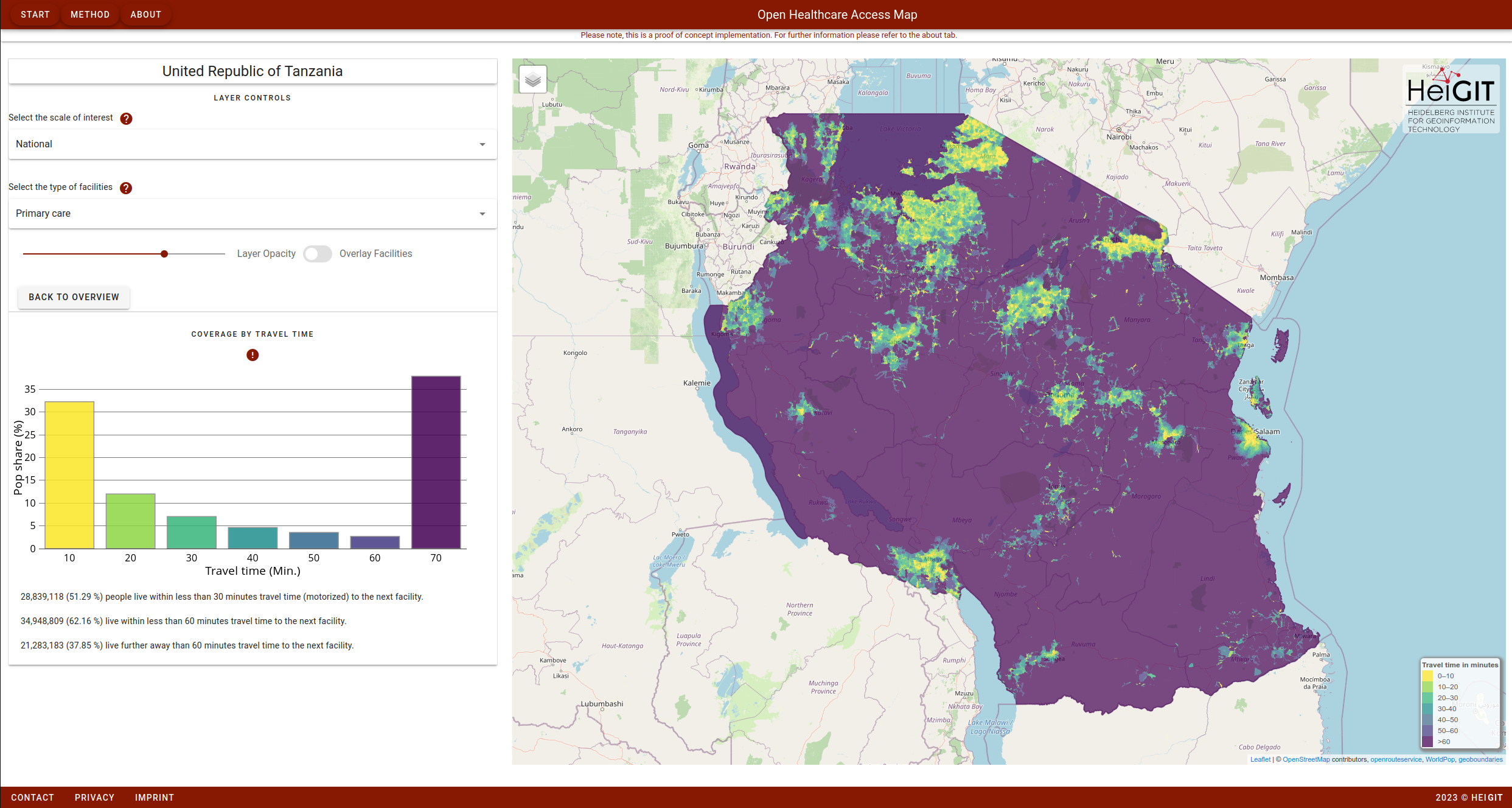
Fig. 44 OpenHealthcareAccessMap provides insights on travel time to healthcare facilities and population coverage at different scales for a variety of countries.#
How many people have access to all pharmacies in Heidelberg within 30 minutes by walking?#
For this exercise, we will follow the methodology proposed utilized in the processing for the OpenHealthcareAccessMap. Areas that can potentially be reached by motorized travel are created using the isochrone service of the openrouteservice. An isochrone basically represents an area that is reachable from location x in time y by means of transport z. Isochrones are based on principles of (road) network analysis. The interaction of facilities, road network, isochrones and population distribution is depicted in the figure on the right. Isochrones are calculated for distinct time intervals of 10 minutes each, up to a maximum of 30 minutes. For each interval, the respective population residing therein is added from WorldPop and then aggregated.
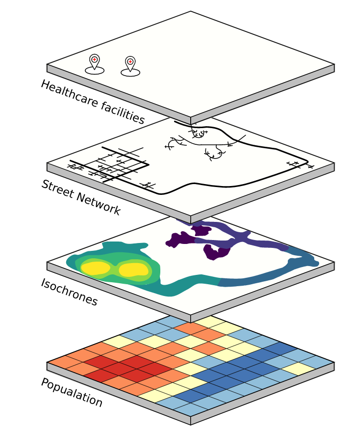
Fig. 45 OpenHealthcareAccessMap provides insights on travel time to healthcare facilities and population coverage at different scales for a variety of countries.#
Get all the datasets#
Preparation#
Check in the OSM Wiki how pharmacies should be mapped in and get the locations of all pharmacies in Heidelberg. Save them as a geojson file (or any other dataformat you prefer). You can use the ohsomeAPI or overpass-turbo for this.
Get familiar with the openrouteservice (ORS) website client and API Playground. Sign up for an ORS api key. You will need this key for this exercise to query the ORS API.
Download the administrative boundary for Heidelberg, e.g. from https://osm-boundaries.com/, and the population distribution for Germany from WorldPop.
Check the completeness of pharmacies#
Plot the temporal evolution of pharmacies mapped in OSM in Heidelberg from 2010 untill today. This should help us to estimate the completeness of pharmacies in OSM for Heidelberg.
Show the steps in Python.
import geopandas as gpd
import matplotlib.pyplot as plt
from ohsome import OhsomeClient

ohsome_client = OhsomeClient()

bpolys = gpd.read_file("data/heidelberg.geojson")

# Define monthly time range and filter.
time = "2008-01-01/2025-01-01/P1M"
filter_str = "amenity=pharmacy"

# Guery ohsome API endpoint to get counts.
response = ohsome_client.elements.count.post(
    bpolys=bpolys,
    time=time,
    filter=filter_str
)

# Get response as dataframe.
results_df = response.as_dataframe()

# Create plot.
plt.figure()
plt.plot(
    results_df["value"]
)

plt.title(f"Temporal evolution of pharmacies in OSM in Heidelberg.")
plt.savefig(f"temporal_evolution.png")
plt.show()
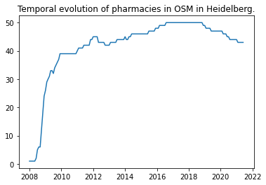
Fig. 46 The curve shows that the number of pharmacies mapped in OSM in Heidelberg has not increased over the past years. Whereas we see an sharp increase between 2008 and 2010 followed by steady increase between 2010 and ~2017, since 2017 the curve seems to be saturated. This is a first indicator that the pharmacies are more or less completely mapped in Heidelberg.#
Derive Physical Access#
Calculate the physical access to pharmacies using the foot-walking profile. Use a maximum range up to 30 minutes and intervals of 5, 15, 30 minutes. Use the ors python package for this. You need make sure to pass the location for each pharmacy as a lat, lon pair to the ORS api.
Show the steps in Python.
import json
import time
from openrouteservice import client

infile = "data/pharmacies_heidelberg.geojson"
with open(infile) as f:
    pharmacies = json.load(f)

# Make sure to get your own openrouteservice api key.
api_key = "your-api-key"
ors_client = client.Client(key=api_key)

# Define the time range in seconds.
time_range = [
    300,  # 5 min
    900,  # 15 min
    1800,  # 30 min
]

# For each pharmacy we will derive the isochrones.
for i, pharmacy in enumerate(pharmacies["features"]):
    # There is a rate limit defined by the ORS API
    # With our "free" api key, we can send max 20 request / minute.
    # Thus we "sleep" here for some time.
    if i > 0 and i % 20 == 0:
        print(f"#{i}: sleeping...")
        time.sleep(60)

    # Get the coordinates from the geometry.
    point_coordinates = pharmacy["geometry"]["coordinates"]

    # Define the request parameters.
    iso_params = {
        "locations": [point_coordinates],
        "profile": "foot-walking",
        "range_type": "time",
        "range": time_range,
    }

    # Do the request.
    request = ors_client.isochrones(**iso_params)
    print(f"successful isochrones request. #{i+1}")

    # Save results into a geojson file.
    outfile = f"data/isochrones_{i}.geojson"
    with open(outfile, 'w') as f:
        json.dump(request, f)
        print(f"saved file: {outfile}")

print("finished")
Note
The ORS API defines a rate limit of 20 requests / minute. Make sure to not send more requests. So in our case here make sure to wait some time after you send 20 requests.
Intersection with Population Raster#
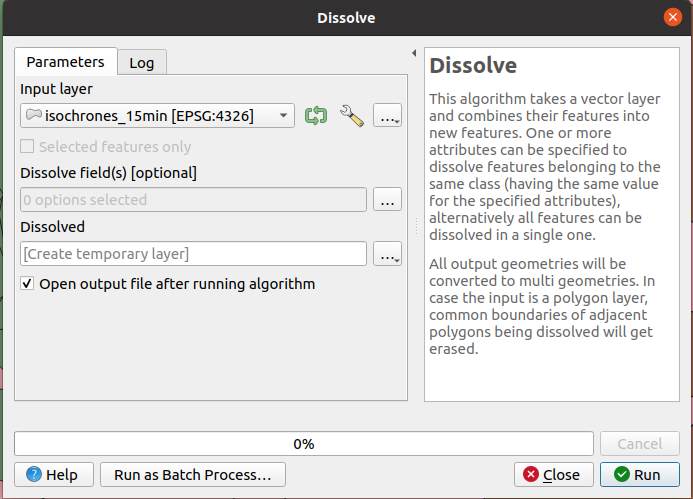
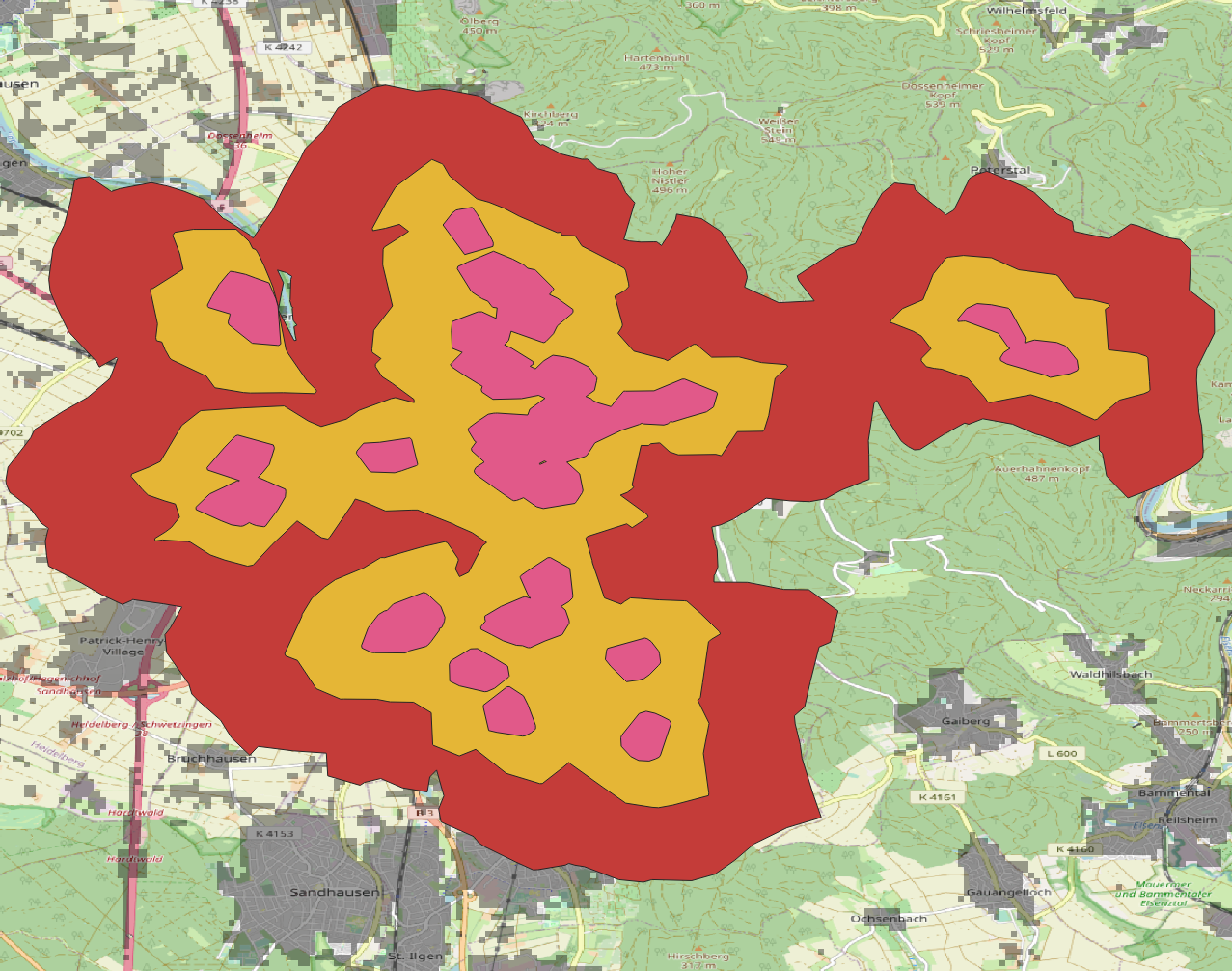
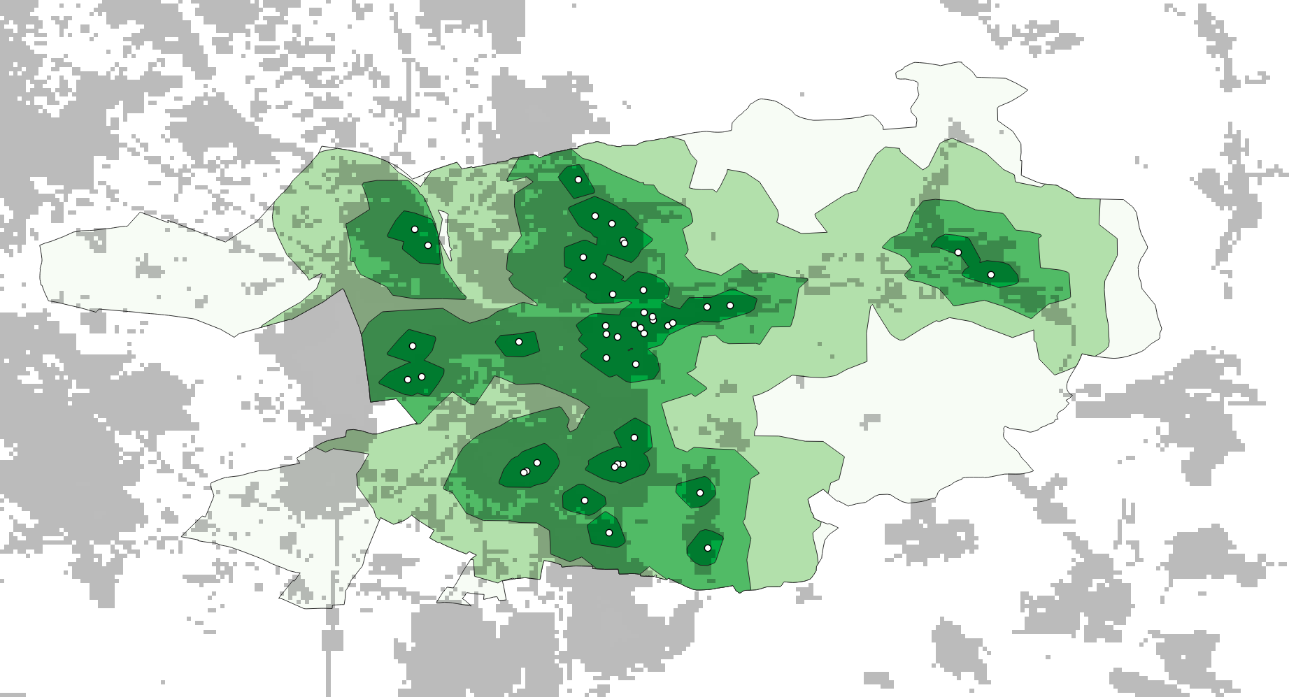
From the ORS api you got individual geojson files representing the isochrones for each pharmacy. Merge all individual files (vector layers) into a single file and the derive the union of all individual isochrones per range. This should give you 3 different polygons each depicting physical access within 5, 15 and 30 minutes.
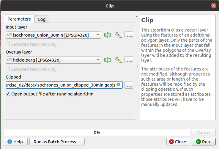
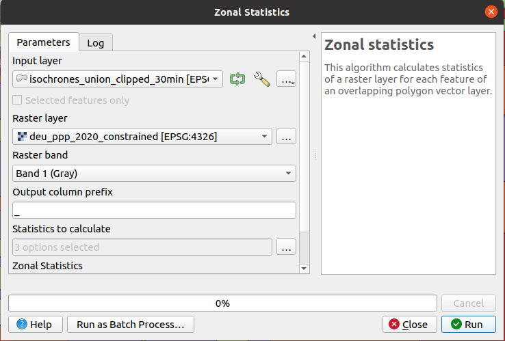
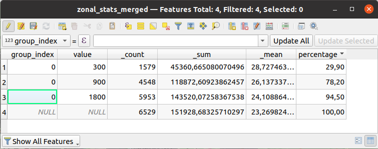
Calculate how many people in Heidelberg have access to pharmacies at the defined ranges. This part of the analysis can be done easily in QGIS. If you like you can try also in Python, but you don’t have to for this exercise.
