Exercise 05: Currentness#
Motivation#
One of OSM’s prominent advantages is that anybody can change the data at any time. This approach stands in contrast to the regular update cycles of traditional map products. However, OSM’s free approach also comes with the downside that there is no regular check if the data is in fact up-to-date. This video shows for the example of Heidelberg, how OSM changes over time. You see that in the beginning new roads are being added and at a later stage roads are updated, e.g. when new attributes are added or the geometry or a road is changed.
An important point in OSM is the currentness of data. After the initial collection process the further maintenance of OSM data is essential for a high quality and up-to-date dataset. Ideally the process of updating the OSM features’ geometries and attributes is carried out continuously, homogeneously, throughout and is not limited to specific feature ([Barron et al., 2014])
Nevertheless, up until now there is only little research about OSM’s temporal quality. [Girres and Touya, 2010] evaluate the actuality of the database relative to changes in the real world for the entire French territory. They find a clear linear correlation between the number of contributors and the recency of OSM objects. [Minghini and Frassinelli, 2019] provide an open source web application to quickly analyze OSM intrinsic quality based on the object history for any specific region.
How up-to-date is OSM data for restaurants with opening hours in Berlin?#
This exercise will deal with the currentness of OSM data in Berlin. Here, we will only look at the OSM data itself and compare how frequently features are updated in OSM. As the opening hours of many restaurants changed during the Covid-19 pandemic, we expect that this should also be reflected in OSM. Hence, we will check to what extent we still see “outdated” data in OSM.
Snapshot based approach#
This part of the exercise will be based on a snapshot of OSM data. The approach here is basically restricted to smaller regions (or datasets) for which you can handle all OSM features in QGIS.
Download osm data through overpass api or ohsome api extraction endpoint#
Make sure to filter for all restaurants in Berlin for which opening_hours have been added as an attribute. In our exercise we will only consider points. Make sure that you download the timestamp when an osm object has been last edited. If your extract contains further attributes, remove them from your extract before you continue with the next steps. You can download the administrative boundary for Berlin through OSM Boundaries.
For the extraction you can use the ohsome API or the overpass API (e.g. through overpass turbo).
Show Code for ohsome API.
import pandas as pd
import geopandas as gpd
from ohsome import OhsomeClient
client = OhsomeClient()

# load the geojson file with geopandas
bpolys = gpd.read_file("../../website/_static/data/berlin.geojson")

# Define which OSM features should be considered.
filter = "amenity=restaurant and opening_hours=* and geometry:point"

# Here we do not set the timestamps parameters.
# This defaults to the most recent timestamp available.
# If you also want to extract the tags, you can use properties=tags,metadata
response = client.elements.geometry.post(
    bpolys=bpolys,
    filter=filter,
    properties="metadata"
)

results_df = response.as_dataframe()

display(results_df)
results_df.plot()

results_df.to_file("../../website/_static/data/berlin_restaurants.geojson", driver='GeoJSON')
Show overpass API query.
[out:json][timeout:25];
// fetch area “berlin” to search in
{{geocodeArea:berlin}}->.searchArea;
// gather results
(
  // query part for: “amenity=restaurant and opening_hours=*”
  node["amenity"="restaurant"]["opening_hours"](area.searchArea);
  way["amenity"="restaurant"]["opening_hours"](area.searchArea);
  relation["amenity"="restaurant"]["opening_hours"](area.searchArea);
);
// make sure to use 'meta' here instead of 'body' to get the timestamp
out meta;
>;
out skel qt;
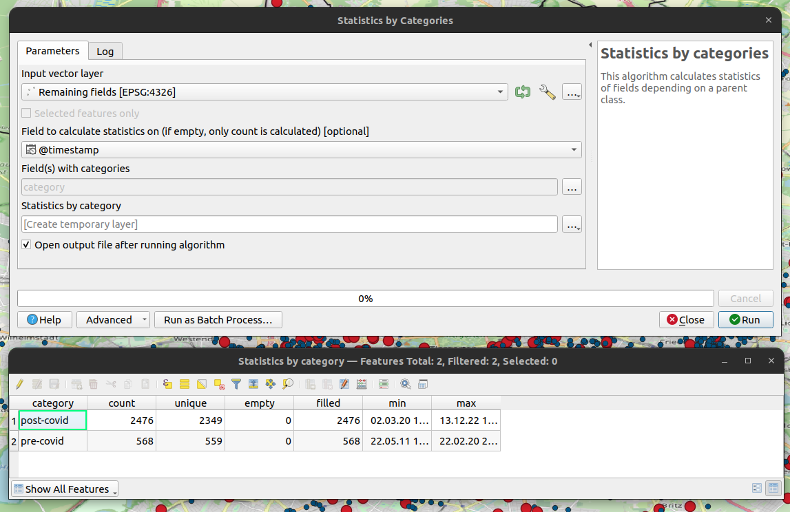
Derive summary statistics for different categories#
Derive summary statistics (min, max, median timestamp) in general and for each of the two categories. Create a histogram of the contributions with Python’s pandas and matplotlib libraries. For this you can use the timestamp values and a bin size of 1 month.
Show Python Code.
import matplotlib.pyplot as plt

# Here we expect that you've already created the dataframe, e.g. by querying the ohsome API.

# make sure to properly set up lastEdit as a timestamp
results_df["@lastEdit"] = pd.to_datetime(results_df["@lastEdit"])

# add a new field 'category' and the default value 'post-covid'
results_df["category"] = 'post-covid'
# update the "category" attribute for all features which have been edited before 2020-03-01
results_df.loc[results_df["@lastEdit"] < "2020-03-01", "category"] = "pre-covid"

# check pandas documentation how to use 'describe()' with timestamps
# https://pandas.pydata.org/pandas-docs/stable/reference/api/pandas.Series.describe.html
display(
    results_df.groupby('category')["@lastEdit"].describe()
)

plt.figure()
# Check the matplotlib.pyplot docu for more information on the parameter
# such as 'rwidth', 'bin' and 'range'.
# https://matplotlib.org/stable/api/_as_gen/matplotlib.pyplot.hist.html
plt.hist(
    results_df["@lastEdit"],
    bins=120,
    range=["2013-01-01", "2025-01-01"],
    rwidth=0.8,
)

median_timestamp = results_df["@lastEdit"].median()
plt.plot(
    [median_timestamp, median_timestamp],
    [0, 700],
    label="median timestamp"
)
plt.ylim([0, 700])
plt.grid()
plt.legend()
plt.show()
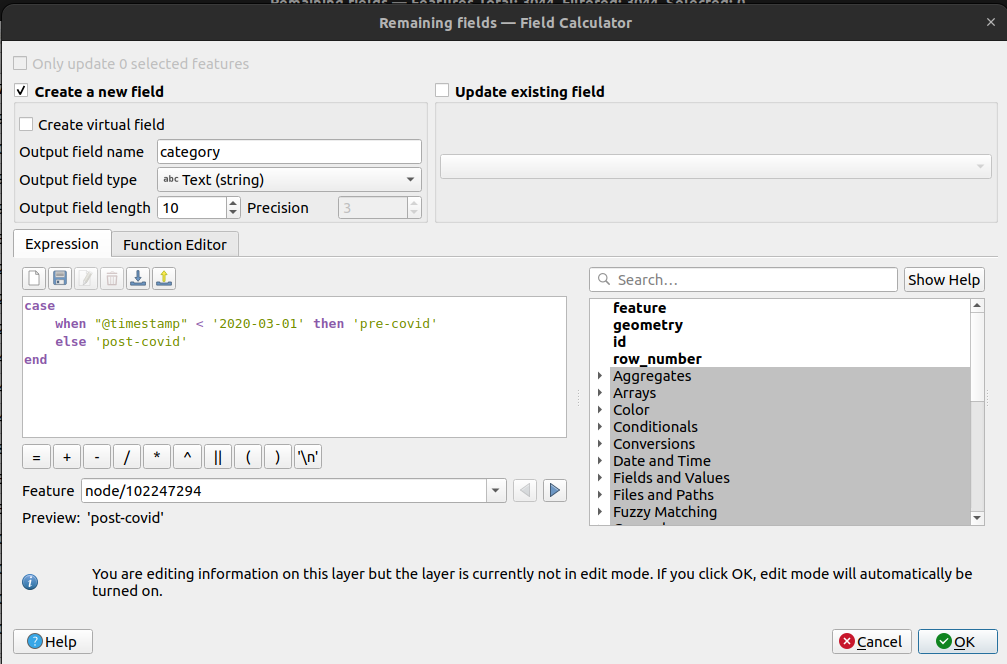
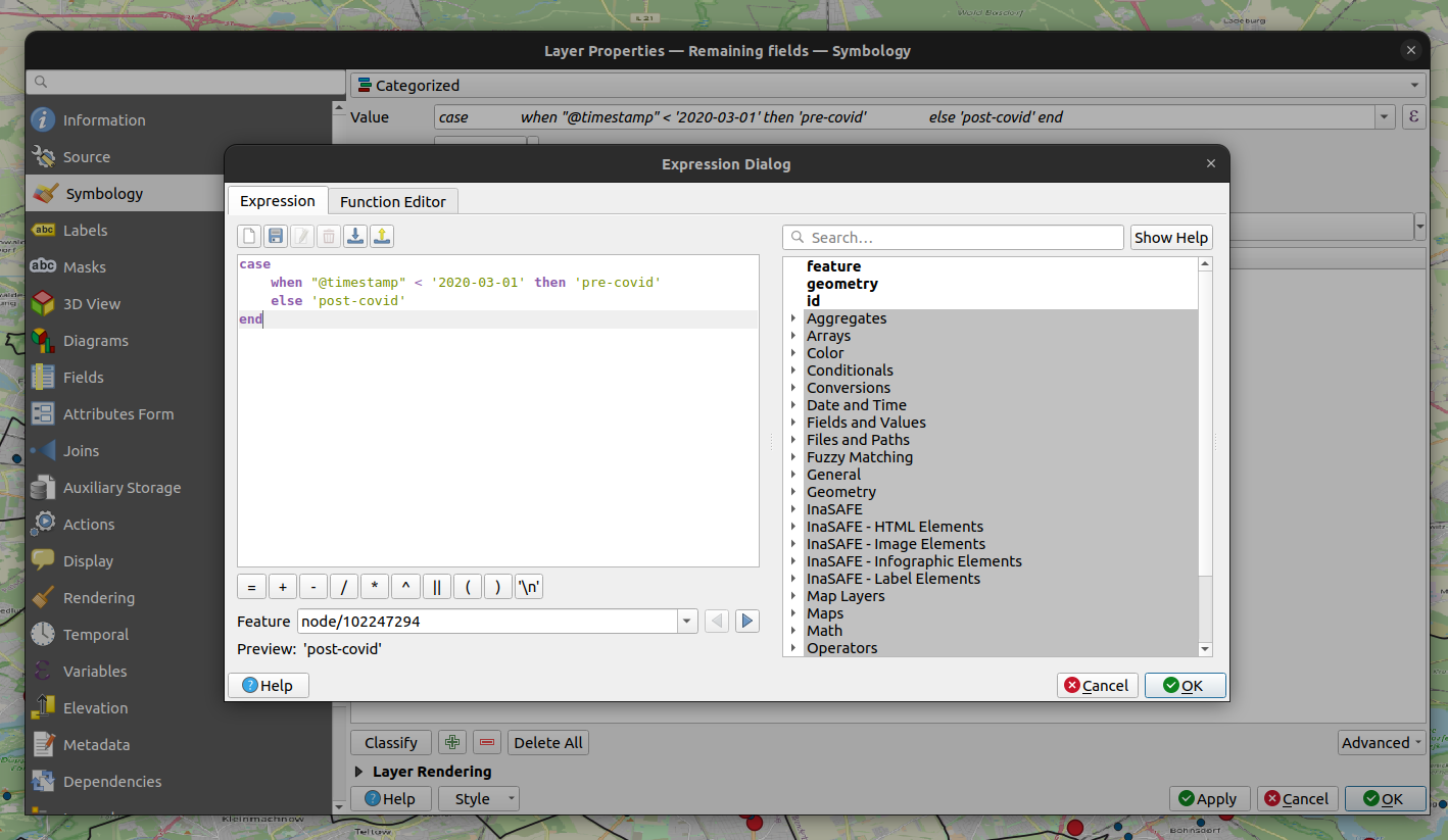
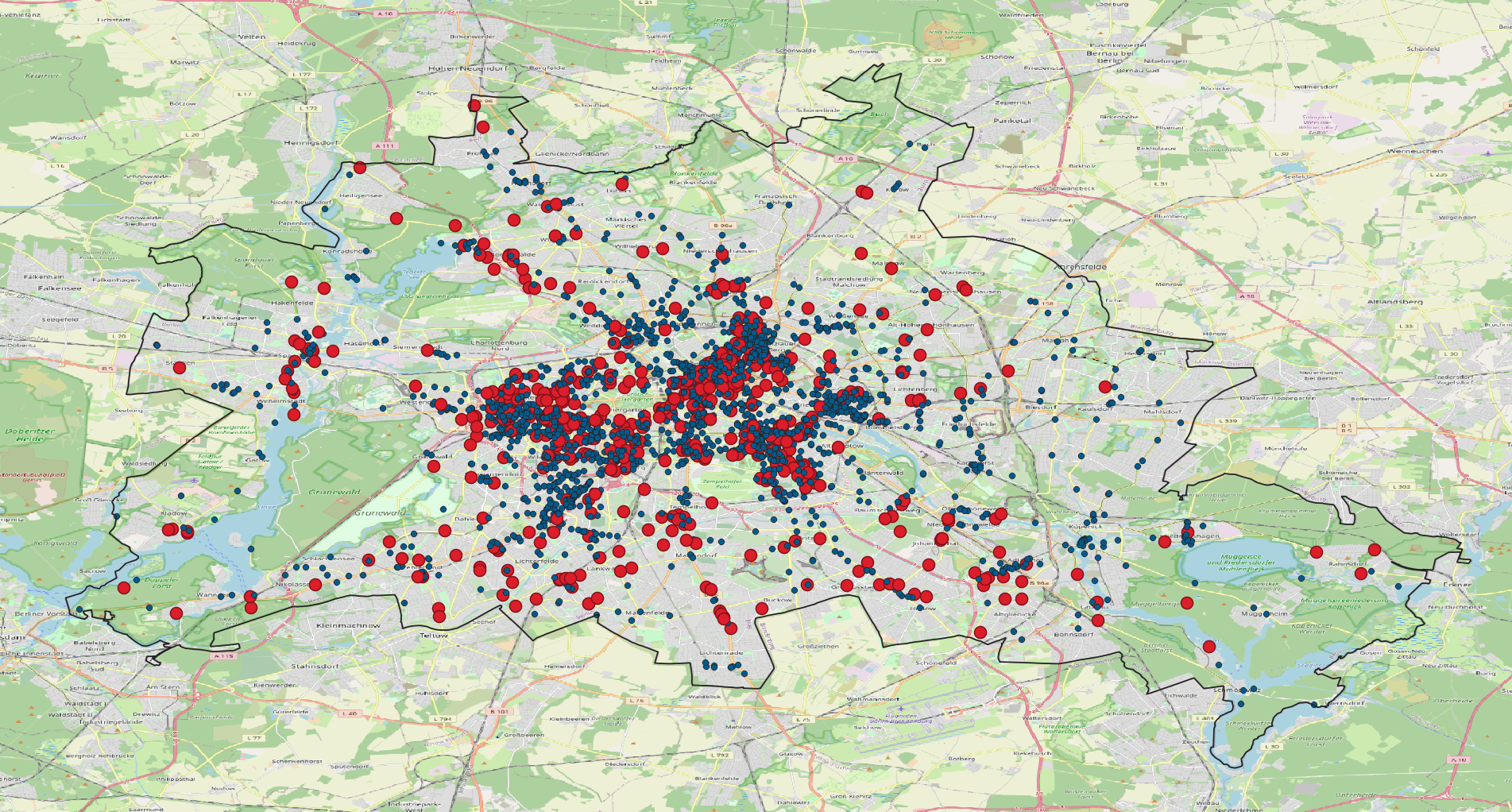
Visualize features based on how “old” they are#
Load your data set in QGIS and style your features according to how old they are. Group features into two classes based on whether they have been edited before or after Covid-19 measures started (~2020-03-01).
Contributions based approach#
For this part of the exercise we will use the OSM changes/contributions as the basis for the analysis. Hence, we get a better overview on overall mapping activity in OSM (compared to only considering the last edit of a feature).
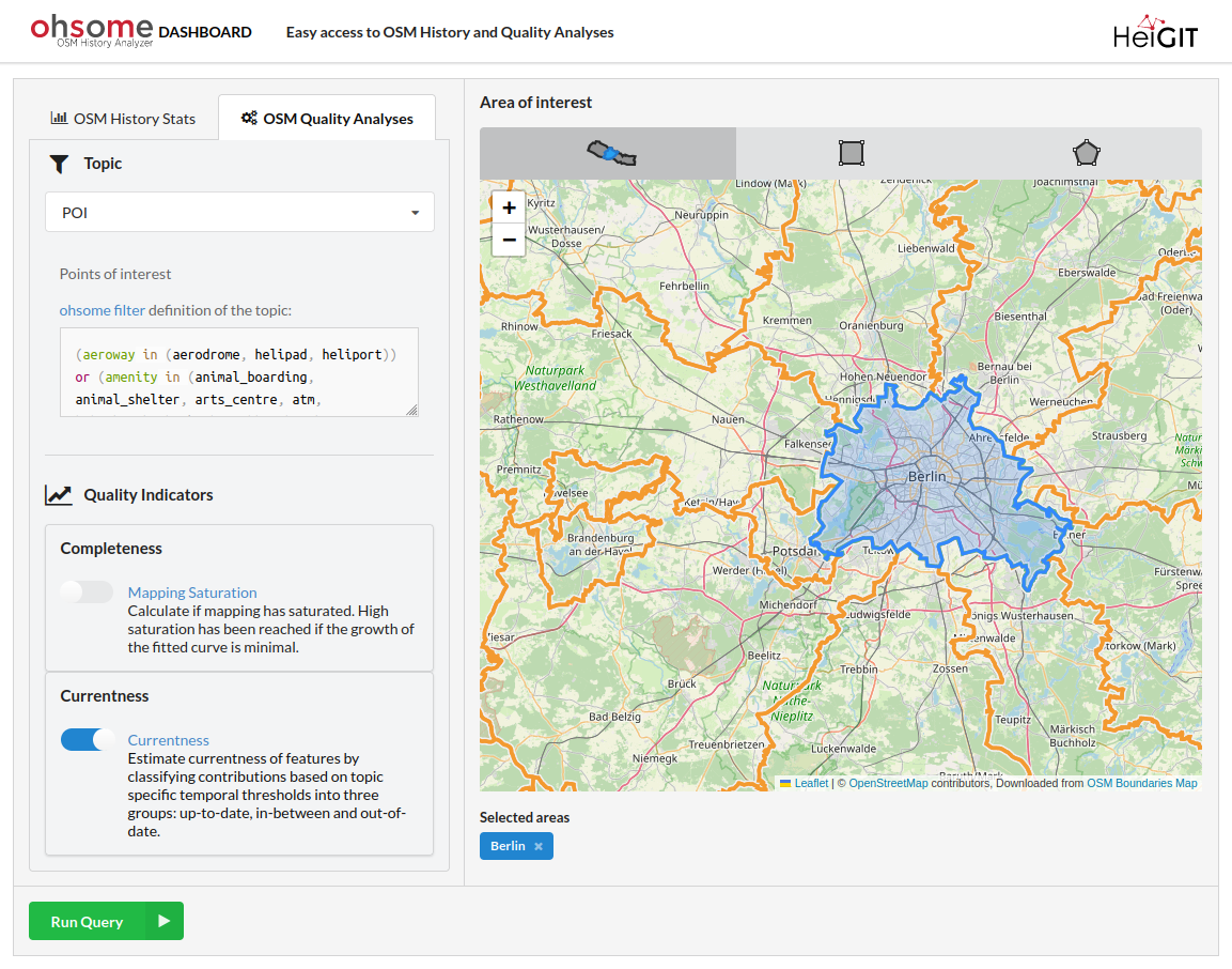
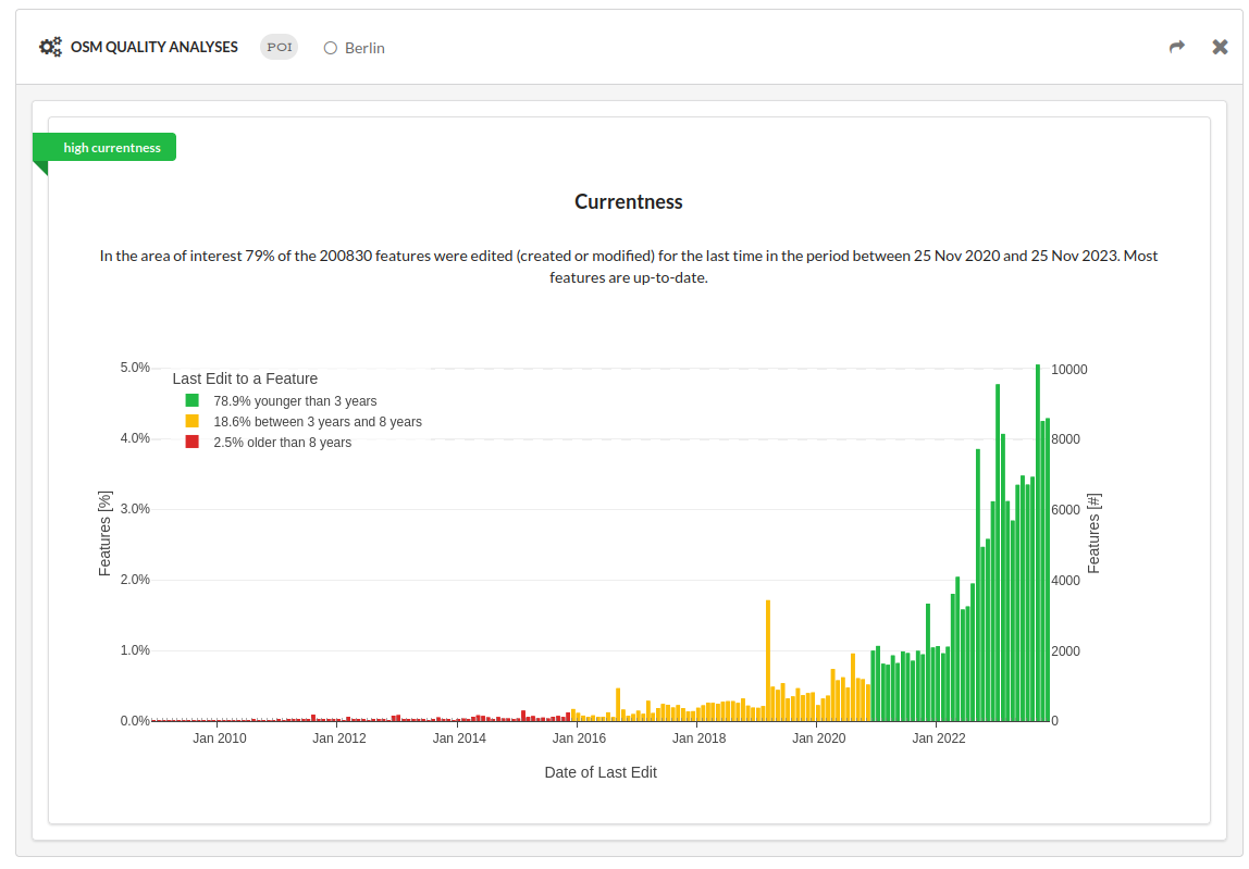
Exploring currentness through the ohsome dashboard#
The ohsome dashboard allows you to calculate various OSM data quality indicators. Currentness is among one of them. Here you can use only pre-defined filters (called “topics”). Explore the currentness of POIs in Berlin.
Derive the number of monthly changes#
Query the ohsome API contributions count endpoint for a monthly time interval between 2013-01-01 and 2022-12-01. Visualize your results in a line plot or bar plot with Python’s matplotlib library. Which month was the one with the highest mapping activity in regard to restaurants with opening hours. (Just to be clear, we consider all edits here which happened for restaurants with opening_hours, but it can be that the change was unrelated to the opening hours.)
Show Python Code.
import pandas as pd
import geopandas as gpd
from ohsome import OhsomeClient
client = OhsomeClient()

# load the geojson file with geopandas
bpolys = gpd.read_file("berlin.geojson")

# Define which OSM features should be considered.
filter = "amenity=restaurant and opening_hours=* and geometry:point"

# Here we set timestamps parameter to a monthly interval
# between 2013-01-01 and 2022-12-01
response = client.contributions.count.post(
    bpolys=bpolys,
    filter=filter,
    time="2013-01-01/2024-11-01/P1M",
)

# display results as dataframe
results_df = response.as_dataframe()
display(results_df)

# plot monthly mapping activity
results_df.reset_index(inplace=True)
plt.figure()
plt.plot(
    results_df["fromTimestamp"],
    results_df["value"],
)
plt.grid()
plt.ylabel("contributions")
plt.plot()