Exercise 03: Positional Accuracy#
Motivation#
At the time when new datasets such as OpenStreetMap emerged, the unstructured and distributed mapping approach raised concerns by various authors and stakeholders. For instance [Haklay, 2010] observe:
In the light of the data collection by amateurs, the distributed nature of data collection and the loose coordination in terms of standards, one of the significant core questions about VGI is ‘how good is the quality of the information that is collected through such activities?’
On the other hand, methods to study spatial data quality aspects, such as positional accuracy, in comparison to other “reference” datasets were already established. In the context of OSM the reference data set is usually obtained from public administration or a commercial datasets.
For example [Goodchild and Hunter, 1997] proposed an extrinsic quality assessment method to measure positional accuracy of linear features which relies on a comparison with a representation (reference dataset) of higher accuracy. Their approach estimates the percentage of the total length of the low accuracy representation that is within a specified distance of the reference representation.
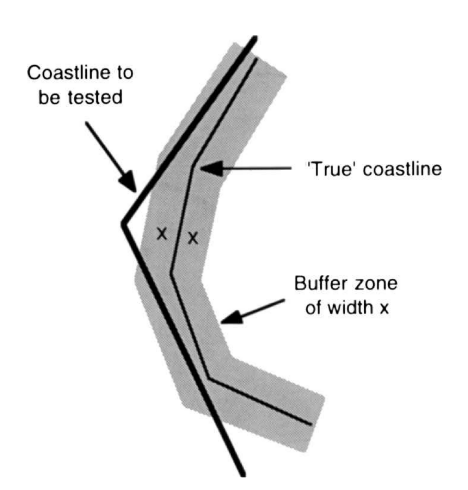
Fig. 5 A buffer of width x around the “true” coastline boundary is intersected with the boundary to be tested, to determine the percentage of coastline lying within the buffer polygon. (source: [Goodchild and Hunter, 1997])#
[Haklay, 2010] carried out the positional accuracy assessment of OSM motorways by comparing agains the Ordnance Survey Meridian dataset. They followed [Goodchild and Hunter, 1997] method and used a buffer distance of 20 meters for the reference dataset and a buffer of 1 meter for the OSM data. Figure Fig. 6 shows their results for OSM data as of 03-2008.
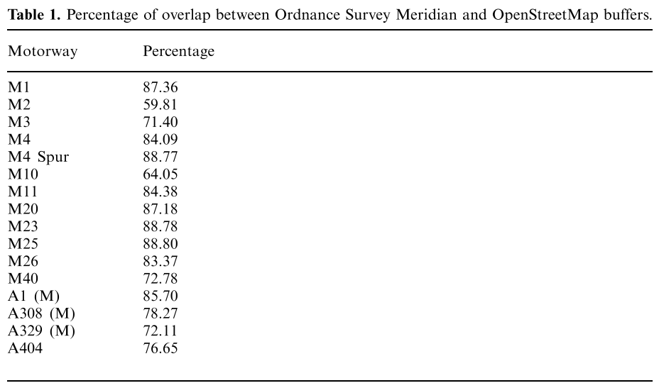
Fig. 6 Overlap between roads features from Ordnance Survey and OpenStreetMap per Motorway (source: [Haklay, 2010])#
What is the current positional accuracy of OSM motorways in the UK?#
In this exercise we want to investigate the positional accuracy of motorways in the UK as of today and will compare our results to the findings of [Haklay, 2010]. For doing so we will apply the buffer methods proposed by [Goodchild and Hunter, 1997].
1. Download Reference Dataset#
The “OS Open Roads” dataset will function as the reference dataset in our analysis. This dataset can be downloaded from the Ordnance Survey Data Hub free of charge. Geopackage will be a good file format for our analysis.
Make sure to properly connect to the Geopackage file in QGIS and don’t just drag and drop the file. (Check the QGIS documentation for more details if needed)
When loading the data in QGIS from the geopackage file you can already filter for motorways. This will facilitate the subsequent steps of the analysis. Use the roadLink layer for this and apply a SQL filter when loading the data.
Show the steps in QGIS.
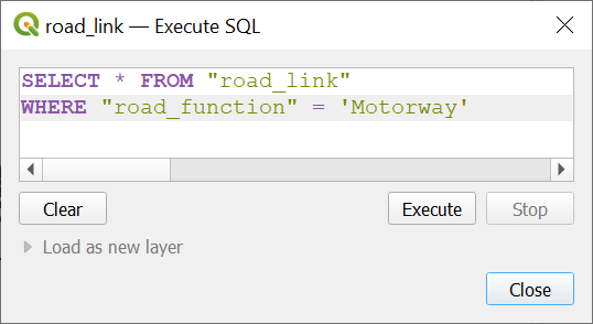
Fig. 7 Filter for motorways in OS Roads roadLink layer#
2. Check Tagging Guidelines and Download OSM Data#
As in previous exercises we will check in the OSM Wiki how motorways (including ramps) should be mapped in OSM. We learn that the following key value combinations are used:
highway=motorwaydescribes a restricted access major divided highway, normally with 2 or more running lanes plus emergency hard shoulder. Equivalent to the Freeway, Autobahn, etc..highway=motorway_linkdescribes the link roads (sliproads/ramps) leading to/from a motorway from/to a motorway or lower class highway. Normally with the same motorway restrictions.
In a second step you can download the OSM motorways for UK, e.g. through GeoFabrik or Overpass Turbo through the QuickOSM plugin in QGIS.
Show the steps in Overpass-Turbo.
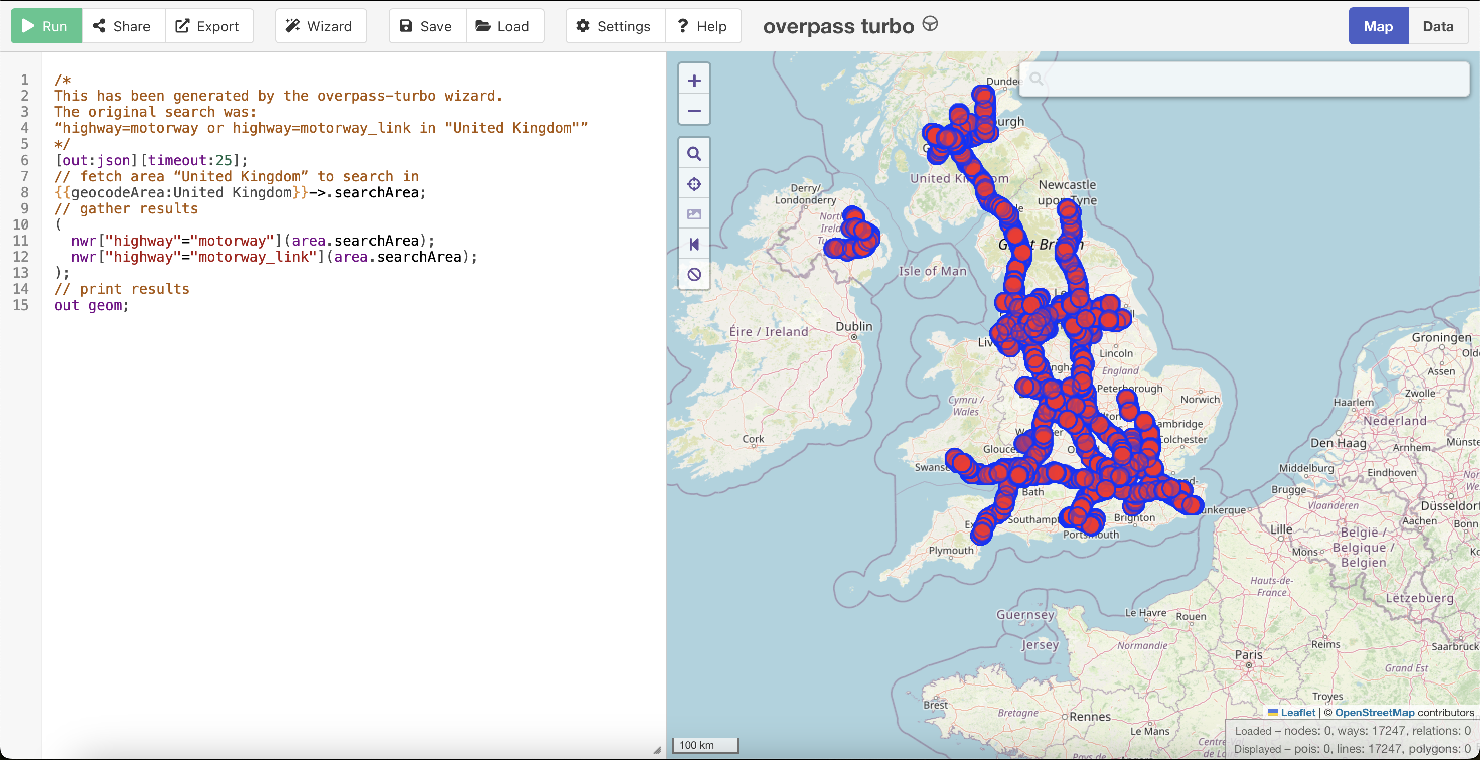
Fig. 8 Download OSM motorways through the Overpass API#
Finally, transform the OSM data in the projection EPSG:27700 (OSGB 1936 / British National Grid).
3. Positional Accuracy of the OSM Motorways in England#
First, apply a buffer of 20 meters to the OS motorways and choose to dissolve the results.
Show the steps in QGIS.
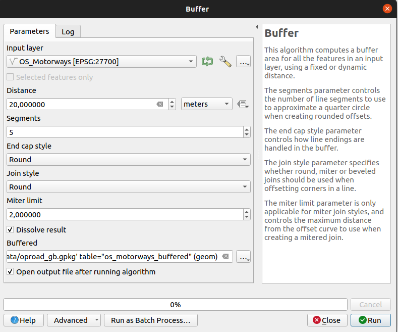
Fig. 9 Buffer OS motorways with 20 meter buffer distance.#
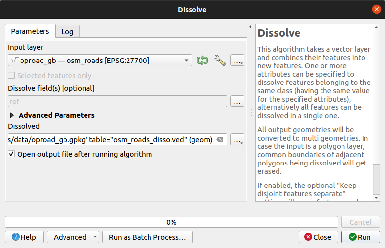
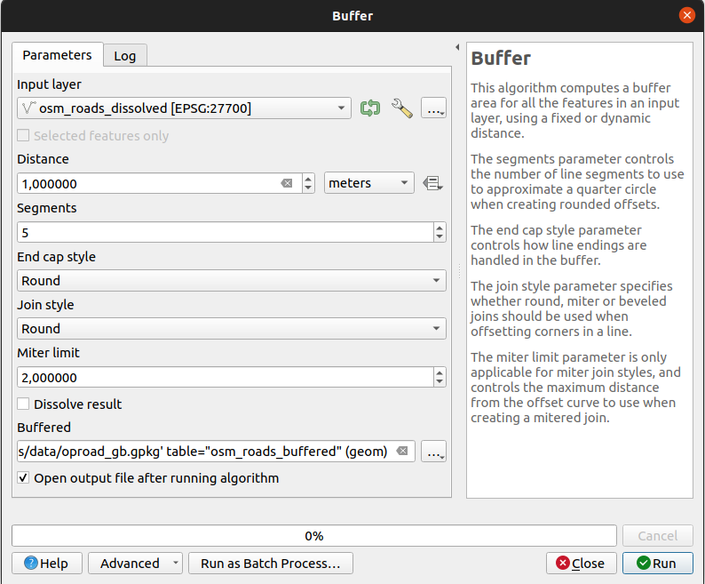
Then, dissolve the OSM motorways by their ref attribute and buffer the resulting layer with 1 meter. This time the buffer results should not be dissolved.
Show the steps in QGIS.
For each dissolved OSM motorway calculate the overall area in square meters.
Show the steps in QGIS.
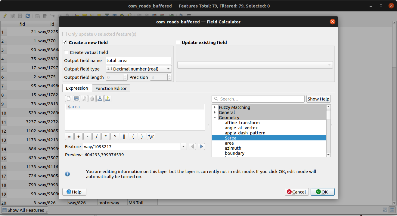
Fig. 12 Calculate area in square meters for the buffered OSM motorways.#
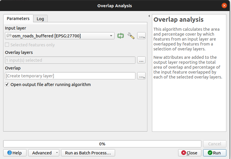
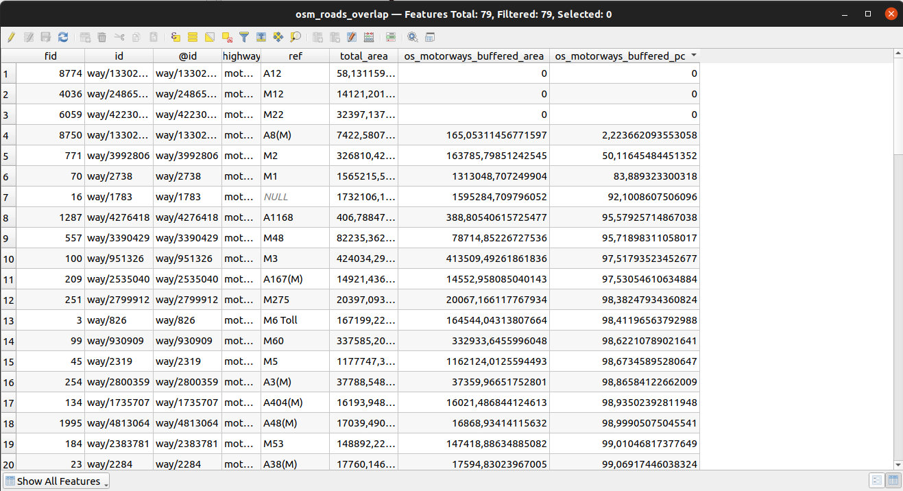
Finally, run the overlap analysis in QGIS to calculate the area that falls within the buffered motorways from OS Open Roads dataset. Calculate the percentage of overall OSM motorway area that lies within the OS Open Roads motorways.