Exercise 04: Completeness#
Motivation#
The completeness of OSM data has been discussed for various applications. Whereas the road network has estimated to be fairly complete, e.g. check work of [Barrington-Leigh and Millard-Ball, 2017], other features such as buildings or point-of-interests (POIs) show a much more scattered coverage. It has been acknowledged that OSM data in general is strongly biased, in part due to a much larger contributor basis in countries in the global North as a consequence of socio-economic inequalities and the digital divide ([Barron et al., 2014, Senaratne et al., 2016]).
Particular attention needs to be paid to data quality, when OSM data is utilized in global studies or to derive global data products. When unaccounted for, spatial bias can lead analysts and researchers to draw general conclusions which are only valid for well-represented (well-mapped) areas. By inadvertently neglecting less well mapped areas in their analyses and datasets, they are in danger of counteracting the overarching goal of the SDGs ensuring that “nobody is left behind”. ([Herfort et al., 2022])
Over a decade ago, [Neis et al., 2011] have analysed the completeness of the OSM street network in relative comparison with a commercial dataset obtained from TomTom. Their research results show that in 2011 OSM provided 27% more data within Germany with regard to the total street network and route information for pedestrians. But, OSM was still missing about 9% of data related to car navigation.
A similar analysis has been conducted by [Haklay, 2010] utilizing the Ordnance Survey Meridian dataset in the UK. They used a grid of 1km x 1km and compared the difference between OSM objects and Meridian objects. For each grid they calculated the OSM road lenght and the Meridian road length and derive the overall length difference. Figure Fig. 15 shows their results and highlights the regions where OSM data is likely to be complete (black areas) and where data is likely to be missing (grey areas).
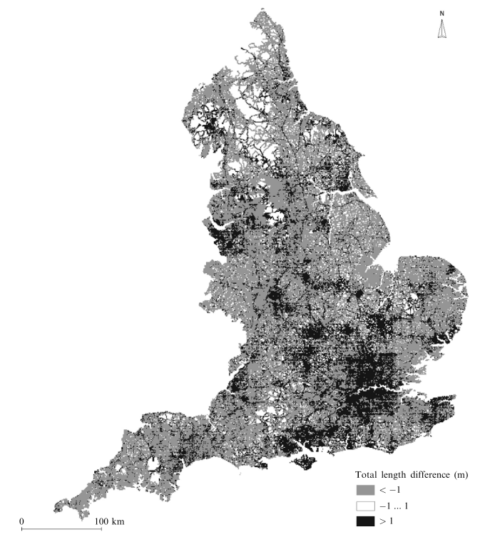
Fig. 15 Difference between OSM road length and OS roads lenght. (source: [Haklay, 2010])#
Such extrinsic analysis, which are based upon a reference dataset, are not applicable in any scenario. Oftentimes a reference dataset of sufficient quality does just not exist. Still, extrinsic completeness analysis can be applied in many regions to understand the completeness of highways or buildings.
What is the current completeness of motorways, A-roads and B-roads in OSM in the UK?#
This exercise will deal with the completeness of the OSM road network in the UK. The analysis will be based upon a comparison of the OSM road length and the OS roads length for grid cells with a cell size of 20 kilometers by 20 kilometers.
1. Download Reference Dataset#
The “OS Open Roads” dataset will function as the reference dataset in our analysis. This dataset can be downloaded from the Ordnance Survey Data Hub free of charge. Geopackage will be a good file format for our analysis.
Note
You can also use the data from Exercise 2.
When loading the data in QGIS from the geopackage file you can already filter for motorways, A-roads and B-roads. This will facilitate the subsequent steps of the analysis. Use the roadLink layer for this and apply a SQL filter when loading the data. Here we can also specify which attributes should be loaded. This can reduce the size of the data quite a lot.
Show the steps in QGIS.
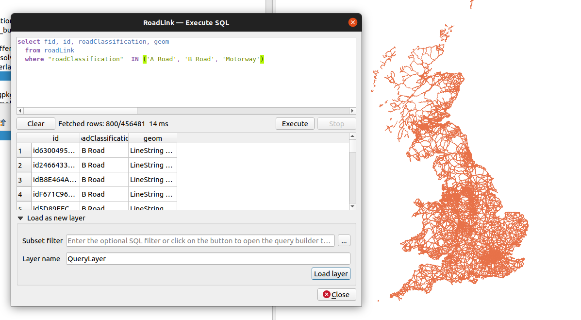
Fig. 16 Filter OS roads for motorways, A-roads and B-roads and specify which attributes should be loaded.#
2. Create grid cells#
There are various types of grids and grid shapes, e.g. point, rectangle or hexagonal grids. Here we use a simple rectangular grid with a cell size of 20 kilometers by 20 kilometers. Use the extent of the OS roads layer to specify the overall extent of the grid.
Show the steps in QGIS.
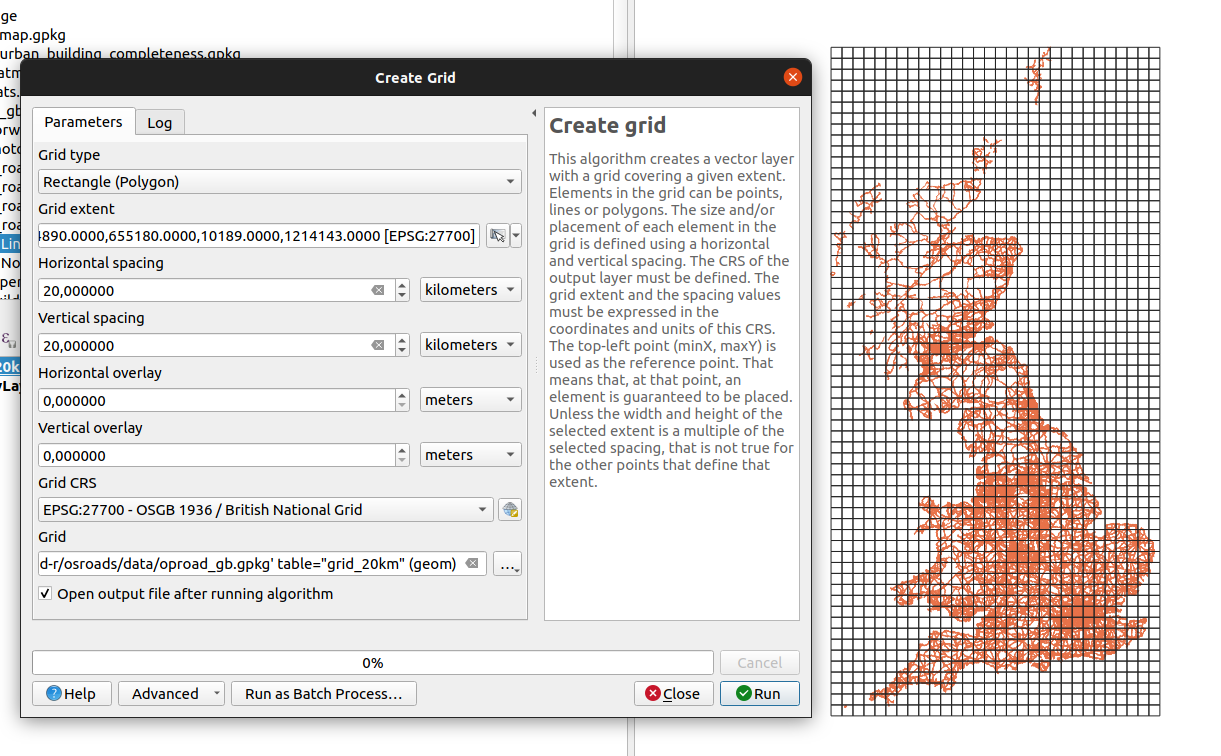
Fig. 17 Create a rectangular grid with a cell size of 20 kilometers.#
3. Aggregate OS roads length per grid cell#
Calculate the sum of the length of all OS open roads per cell in QGIS. This is a relatively “expensive” computation, so you might pick only a sample of 10 cells and not all cells to speed up things.
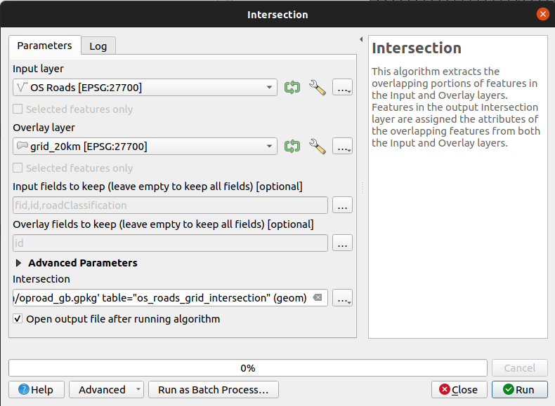
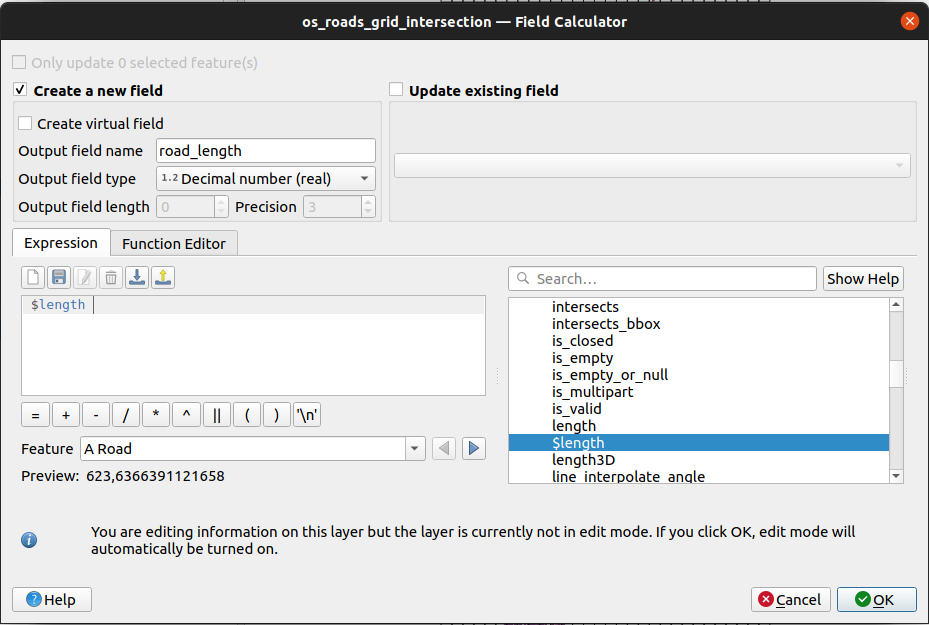
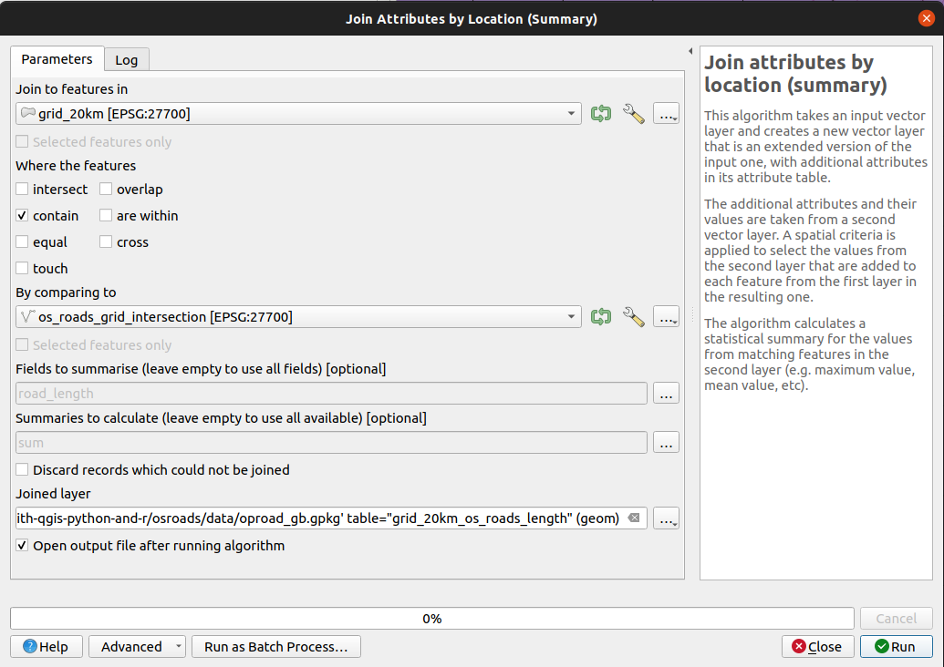
First, intersect the roads layer and the grid layer. This will provide you with the grid ID value for each road segment. Then calculate the length of each road segment in meters. Finally, sum up the road length values per grid cell, e.g. by joining the sum of the road length to the grid or by using the Statistics by Categories tool.
Show the steps in QGIS.
Export your file as a geojson file and make sure to use EPSG:4326 as the coordinate system. This is the one supported by the ohsome API and thus needed in the next step of the analysis.
Note
You can download a file containing the stats for all cells.
4. Calculate OSM road length and derive completeness#
In theory, you could follow the same workflow as for the OS roads dataset: Download OSM data, intersect with the grid, derive the length per OSM road segment and finally sum up values per grid cell. Nevertheless, we want to use a different approach here which utilizes the ohsome API and simplifies the analysis to sending a single API request.
Define which OSM features should be considered.You can select a subset of the OSM data using the following filter condition: highway in (motorway, motorway_link, trunk, trunk_link, primary, primary_link, secondary, secondary_link) and type:way.
For the analysis we will use the elements/length/groupByBoundary endpoint of the ohsome API. The 20km grid will function as our input layer for this query.
Compare the road length from Ordnance Survey and for OSM for your sample regions in two different ways:
Derive the length difference per cell. (
OSM_roads_length - OS_roads_length)Derive the ratio between OSM road length and OS road length. (
OSM_roads_length / OS_roads_length)
Show Code.
# to install in google colab use
# %pip install ohsome
# %pip install numpy==1.24.0

import pandas as pd
import geopandas as gpd
import matplotlib.pyplot as plt
from ohsome import OhsomeClient
client = OhsomeClient()


# load the geojson file with geopandas
bpolys = gpd.read_file("/content/grid_with_os_road_stats.geojson")

bpolys.set_index("fid", inplace=True)

# Define which OSM features should be considered.
filter_roads = "highway in (motorway, motorway_link, trunk, trunk_link, primary, primary_link, secondary, secondary_link) and type:way"

# Here we do not set the timestamps parameters.
# This defaults to the most recent timestamp available.
response = client.elements.length.groupByBoundary.post(
    bpolys=bpolys,
    filter=filter_roads
)

# display results as dataframe
results_df = response.as_dataframe()

# reset the index
results_df.reset_index(inplace=True)

# Convert "boundary" column to int64
results_df["boundary"] = results_df["boundary"].astype(int)

# Join input DataFrame and results DataFrame on the "id" column from bpolys and the "boundary" column from results_df
join_df = bpolys.merge(results_df, left_index=True, right_on="boundary")


# calculate difference between OS road length and OSM road length
join_df["difference"] = join_df["value"] - join_df["road_length_sum"]

# calculate ratio between OS road length and OSM road length
# here we calculate to what extend OSM covers the OS roads
# <1 => less OSM roads than OS
# 1 => OSM roads and OS roads are almost the same
# >1 => more OSM roads than OS
join_df["ratio"] = join_df["value"] / join_df["road_length_sum"]

join_df.to_file("/content/grid_20km_with_osm_stats_4326.geojson", driver='GeoJSON')
5. Visualize your results#
Create a map overview how complete OSM road data is now. Use QGIS or python for this.